How To Color Alternate Rows In Excel Automatically
“`html
Automatically Coloring Alternate Rows in Excel: A Comprehensive Guide
Manually coloring alternate rows in Excel can be tedious, especially with large datasets. Fortunately, Excel provides powerful tools to automate this process, making your spreadsheets more readable and visually appealing. This guide explores different methods to achieve this, catering to various Excel versions and complexity requirements.
Method 1: Using Conditional Formatting (The Recommended Approach)
Conditional formatting is the most versatile and dynamic method for coloring alternate rows. It automatically applies formatting based on a formula, ensuring that your spreadsheet remains consistently formatted even after adding or deleting rows.
Steps:
- Select Your Data Range: Click and drag your mouse to select the range of cells you want to apply the alternate row coloring to. This should include all the columns and rows you want formatted. Be mindful of header rows; decide if you want them included in the alternating pattern.
- Access Conditional Formatting: Go to the “Home” tab on the Excel ribbon. In the “Styles” group, click on “Conditional Formatting.”
- Create a New Rule: From the dropdown menu, select “New Rule…” This opens the “New Formatting Rule” dialog box.
- Choose “Use a formula to determine which cells to format”: In the “Select a Rule Type” section, choose the last option: “Use a formula to determine which cells to format.”
- Enter the Formula: In the “Format values where this formula is true:” box, you’ll need to enter a formula. The formula will determine whether a row is even or odd.
Here are two commonly used formulas:
- Using the MOD and ROW functions (Most reliable and recommended):
=MOD(ROW(),2)=0Explanation:
ROW(): This function returns the row number of the current cell. If you want to start coloring from row 1, then using `ROW()` directly is fine. If you want to account for a header row, you may need to adjust the formula.MOD(ROW(),2): The `MOD` function returns the remainder after dividing `ROW()` by 2. So, it will return 0 for even row numbers and 1 for odd row numbers.=0: This part of the formula checks if the remainder is equal to 0. If it is, the formula returns TRUE, and the formatting will be applied to that row. Therefore this will color even rows. If you want to color odd rows, use `MOD(ROW(),2)=1`.
- Using the ISODD and ISEVEN functions (simpler to read):
=ISODD(ROW())or=ISEVEN(ROW())Explanation:
ISODD(ROW()): This function directly checks if the row number is odd. It returns TRUE if the row number is odd and FALSE if it is even.ISEVEN(ROW()): This function directly checks if the row number is even. It returns TRUE if the row number is even and FALSE if it is odd.
Choose either `ISODD` or `ISEVEN` depending on whether you want to color the odd or even rows.
Important Note regarding Relative and Absolute References: In conditional formatting formulas, be mindful of relative and absolute references. In this case, we *want* the `ROW()` function to adjust as the conditional formatting is applied to each row. Therefore, do *not* use `$` symbols to make the row number absolute (e.g., `$A$1`). The formula should remain `ROW()`.
- Using the MOD and ROW functions (Most reliable and recommended):
- Set the Formatting: Click the “Format…” button. This opens the “Format Cells” dialog box.
- Choose a Fill Color: Go to the “Fill” tab. Select the background color you want to use for the alternate rows. Consider using light, subtle colors for readability.
- Other Formatting Options (Optional): You can also customize other formatting options, such as font color, font style, borders, etc., under the other tabs in the “Format Cells” dialog box.
- Apply the Rule: Click “OK” to close the “Format Cells” dialog box and then click “OK” again to close the “New Formatting Rule” dialog box.
Advantages of Conditional Formatting:
- Dynamic: The formatting automatically adjusts when you add, delete, or sort rows.
- Easy to Update: You can easily change the formatting or the formula if needed.
- Clear Rules Management: Excel’s Conditional Formatting Rules Manager allows you to view, edit, and delete your conditional formatting rules in one place.
Managing Conditional Formatting Rules:
To access the Conditional Formatting Rules Manager:
- Select any cell within the data range where the conditional formatting is applied.
- Go to the “Home” tab, click on “Conditional Formatting,” and then select “Manage Rules…”
In the Rules Manager, you can:
- Edit a Rule: Select a rule and click “Edit Rule…”
- Delete a Rule: Select a rule and click “Delete Rule.”
- Change the Rule Order: If you have multiple conditional formatting rules applied to the same cells, the order in which they are listed determines which rule takes precedence. Use the up and down arrows to change the order.
- View Rules for: You can choose to view rules applied to the “Current Selection” or “This Worksheet.”
Method 2: Using Tables (Another Excellent Option)
Excel Tables provide a built-in feature to automatically color alternate rows, known as “banded rows.” This is a quick and easy way to achieve the desired effect without using formulas.
Steps:
- Select Your Data Range: Select the data range you want to format as a table, including headers if you have them.
- Insert a Table: Go to the “Insert” tab on the Excel ribbon. Click on “Table.” Alternatively, you can use the keyboard shortcut `Ctrl + T`.
- Confirm the Range: A “Create Table” dialog box will appear. Verify that the selected range is correct. If you have headers, make sure the “My table has headers” checkbox is selected.
- Click OK: Click “OK” to create the table.
- Table Styles: Once the table is created, the “Table Design” tab will appear on the ribbon. In the “Table Styles” group, you’ll find various pre-defined table styles. Many of these styles include banded rows by default.
- Enable Banded Rows (If Necessary): If the current table style doesn’t have banded rows, or if you want to customize them, in the “Table Style Options” group on the “Table Design” tab, ensure that the “Banded Rows” checkbox is selected.
- Customize Table Style (Optional): You can further customize the table style by selecting a different style from the “Table Styles” gallery or by modifying the existing style by right-clicking on a style and choosing “Modify Table Style…”
Advantages of Using Tables:
- Simple and Quick: It’s a very straightforward process.
- Automatic Formatting: Excel handles the alternate row coloring automatically.
- Dynamic: The formatting adjusts when you add or delete rows or columns within the table.
- Built-in Features: Tables offer other useful features such as filtering, sorting, and automatic calculation of totals.
Disadvantages of Using Tables:
- Less Flexibility than Conditional Formatting: While you can customize the table style, the banding pattern options are more limited compared to the fine-grained control offered by conditional formatting formulas.
Method 3: Manual Coloring (Not Recommended for Large Datasets)
While not recommended for large datasets, manual coloring can be used for small, static spreadsheets.
Steps:
- Select the First Row to be Colored: Click on the row number to select the entire row.
- Apply the Fill Color: Go to the “Home” tab. In the “Font” group, click the dropdown arrow next to the “Fill Color” (paint bucket) icon and select a color.
- Select the Third Row (Skipping one): Click on the row number to select the third row.
- Apply the Same Fill Color: Click the “Fill Color” icon again. Excel usually remembers the last used color.
- Use the Format Painter: Select both the first and third row (or as many manually colored rows as you like to establish the pattern). Click on the “Format Painter” icon on the Home tab (it looks like a paintbrush).
- Paint the Remaining Rows: Click and drag the Format Painter down the rows you want to format. The format will be applied in the alternating pattern you established.
Disadvantages of Manual Coloring:
- Tedious and Time-Consuming: Very inefficient for large datasets.
- Static: The formatting doesn’t automatically adjust if you add or delete rows. You’ll need to manually re-apply the formatting.
- Error-Prone: Easy to make mistakes and skip rows.
Choosing the Right Method
The best method for coloring alternate rows depends on your specific needs:
- Conditional Formatting: The most flexible and dynamic option, especially suitable for large datasets that are frequently updated. Requires a bit of formula knowledge.
- Tables: A quick and easy way to add alternate row coloring, suitable for datasets that benefit from other table features. Less flexible than conditional formatting in terms of customization.
- Manual Coloring: Only suitable for small, static datasets where you don’t anticipate any changes. Generally not recommended.
Conclusion
Excel provides several options for automatically coloring alternate rows. Conditional formatting offers the most flexibility and dynamic behavior, while tables provide a simpler and quicker solution with built-in banding. Choose the method that best suits your needs and enjoy more readable and visually appealing spreadsheets!
“`
 700×574 apply color alternate rows columns excel benisnous from benisnous.com
  824×438 automatically color alternating rowscolumns excel from www.extendoffice.com
  0 x 0 apply color alternate rows columns excel from www.thewindowsclub.com
  1280×600 automatically color alternating rows excel microsoft office from ms-office.wonderhowto.com
  768×489 alternate row color excel alternate row color excel from www.educba.com
  889×500 color alternate lines excel excel grid from exceloffthegrid.com
 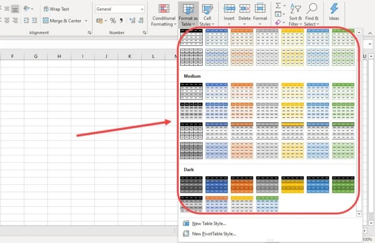 768×498 shade alternate rows columns microsoft excel from candid.technology
  515×517 add alternate row color excel methods from www.wallstreetmojo.com