How To Sum Values Based On Text In Excel
“`html
Summing Values Based on Text in Excel
Excel is a powerful tool for data analysis, and one of its most useful capabilities is summing values based on specific criteria. When dealing with textual data, the ability to conditionally sum values based on matching text is essential. This document explores various methods for achieving this in Excel, ranging from simple functions to more advanced techniques.
1. The SUMIF Function
The most straightforward way to sum values based on text is using the SUMIF function. This function takes three arguments:
- Range: The range of cells containing the text criteria.
- Criteria: The text you want to match. This can be a literal string, a cell reference containing the text, or a wildcard.
- Sum_range: The range of cells containing the values you want to sum. This range must be the same size as the ‘Range’ argument.
The syntax is as follows:
=SUMIF(range, criteria, sum_range)
Example:
Imagine you have a table of sales data with columns “Product” and “Sales Amount”. To sum the sales amount for all entries where the product is “Apple”, you would use:
=SUMIF(A:A, "Apple", B:B)
Here, A:A is the “Product” column, "Apple" is the text criterion, and B:B is the “Sales Amount” column.
Using Cell References:
Instead of hardcoding the text criterion, you can use a cell reference. If cell D1 contains the text “Apple”, the formula becomes:
=SUMIF(A:A, D1, B:B)
This makes the formula more dynamic, allowing you to change the criteria by simply updating the value in cell D1.
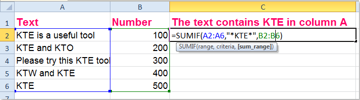
Wildcards:
SUMIF supports wildcard characters for partial text matching:
- *: Represents any number of characters.
- ?: Represents a single character.
For example, to sum sales amounts for products starting with “A”, you would use:
=SUMIF(A:A, "A*", B:B)
To sum sales amounts for products with “pple” anywhere in the name, use:
=SUMIF(A:A, "*pple*", B:B)
2. The SUMIFS Function
SUMIFS is an extension of SUMIF that allows you to specify multiple criteria. This is useful when you need to sum values based on multiple textual conditions.
The syntax is:
=SUMIFS(sum_range, criteria_range1, criteria1, [criteria_range2, criteria2], ...)
- sum_range: The range containing the values to sum.
- criteria_range1: The first range to evaluate against a criterion.
- criteria1: The first criterion.
- [criteria_range2, criteria2], …: Optional additional ranges and criteria. You can add up to 127 range/criteria pairs.
Example:
Suppose you have a table with “Product”, “Region”, and “Sales Amount”. To sum the sales amounts for “Apple” in the “East” region, you would use:
=SUMIFS(C:C, A:A, "Apple", B:B, "East")
Here, C:C is the “Sales Amount” column, A:A is the “Product” column, "Apple" is the product criterion, B:B is the “Region” column, and "East" is the region criterion.
Using Cell References with SUMIFS:
Similar to SUMIF, you can use cell references for the criteria in SUMIFS.
If cell D1 contains “Apple” and cell E1 contains “East”, the formula becomes:
=SUMIFS(C:C, A:A, D1, B:B, E1)
Wildcards with SUMIFS:
SUMIFS also supports wildcard characters, allowing for more flexible criteria matching.
3. The SUM and IF Array Formula (Legacy, but sometimes useful)
Before SUMIF and SUMIFS, array formulas were commonly used to achieve conditional summing. While less efficient and more complex to understand, they are still a viable option, especially when dealing with older Excel versions or needing very specific logic that isn’t easily handled by the other functions.
The general structure is:
=SUM(IF(criteria_range=criteria, sum_range))
Important: After entering this formula, you must press Ctrl + Shift + Enter to enter it as an array formula. Excel will automatically add curly braces {} around the formula to indicate it’s an array formula (do not type the curly braces yourself).
Example:
To sum the sales amount for “Apple” using an array formula, you would use:
=SUM(IF(A:A="Apple", B:B))
Remember to press Ctrl + Shift + Enter after typing the formula.
Multiple Criteria with Array Formulas:
You can combine multiple criteria using logical operators within the IF function.
To sum the sales amount for “Apple” in the “East” region, you would use:
=SUM(IF((A:A="Apple")*(B:B="East"), C:C))
Again, press Ctrl + Shift + Enter after entering the formula.
The * operator acts as an “AND” condition. Each condition (e.g., A:A="Apple") results in an array of TRUE and FALSE values. Multiplying these arrays together results in 1 (representing TRUE) only when both conditions are TRUE, and 0 (representing FALSE) otherwise.
To use an “OR” condition, use the + operator instead of *.
4. Using Helper Columns
In some cases, creating a helper column can simplify the summation process, especially when dealing with complex criteria or needing to perform multiple summations with slightly different conditions.
Example:
Suppose you need to sum sales amounts for products that contain the word “Fruit” but exclude “Grapefruit”.
- Create a helper column (e.g., Column C) with a formula like:
=IF(AND(ISNUMBER(SEARCH("Fruit", A2)), NOT(ISNUMBER(SEARCH("Grapefruit", A2)))), 1, 0)This formula checks if “Fruit” is present in the product name and “Grapefruit” is not. It returns 1 if both conditions are met, and 0 otherwise. - Use
SUMIFto sum the “Sales Amount” (Column B) where the helper column (Column C) equals 1:=SUMIF(C:C, 1, B:B)
This approach breaks down the complex logic into smaller, more manageable steps.
5. Power Query (Get & Transform Data)
For more complex data manipulation and aggregation, especially with large datasets or data from external sources, Power Query offers a robust solution. Power Query allows you to filter data based on text criteria and then group and sum the desired values.
Steps:
- Select your data and go to
Data > From Table/Rangeto load the data into the Power Query Editor. - Use the
Filteroption on the column containing the text criteria to filter the rows based on your desired text (e.g., “Text Filters > Contains”). You can use multiple filters for multiple criteria. - Go to
Group Byin theTransformtab. - Select the column you want to group by (e.g., “Product”).
- Add a new aggregation by selecting the “Sales Amount” column and choosing “Sum” as the operation.
- Click “OK”.
- Go to
Home > Close & Loadto load the transformed data back into Excel.
Power Query offers greater flexibility and performance when dealing with complex transformations and large datasets compared to traditional Excel formulas.
Conclusion
Excel provides several methods for summing values based on text criteria. SUMIF and SUMIFS are the most commonly used functions for straightforward scenarios. Array formulas offer more flexibility for complex logic but are generally less efficient. Helper columns can simplify complex criteria evaluation. For advanced data manipulation and large datasets, Power Query provides a powerful and efficient solution. Choosing the appropriate method depends on the complexity of the criteria, the size of the dataset, and the desired level of flexibility.
“`
 714×198 sum values based text criteria excel from www.extendoffice.com
  1200×630 sum text values numbers excel formula exceljet from exceljet.net
 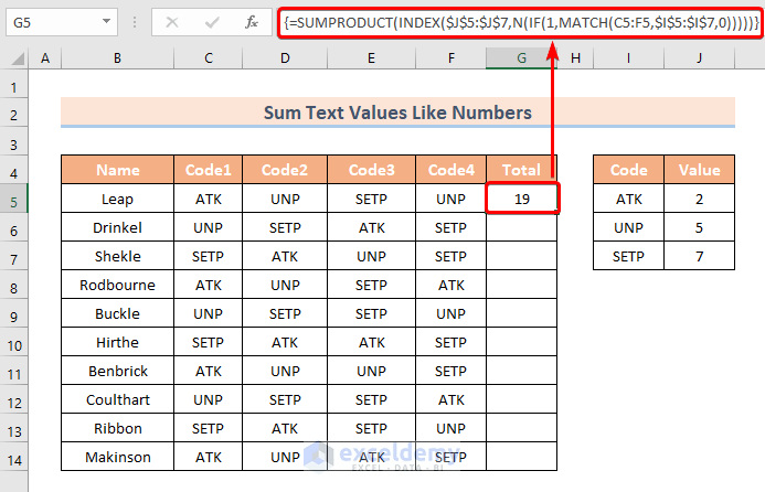 693×446 sum text values numbers excel methods from www.exceldemy.com
  944×708 excel tutorial sum text values excel excel dashboardscom from dashboardsexcel.com
  1024×576 sum cells based text numbers excelnotes from excelnotes.com
 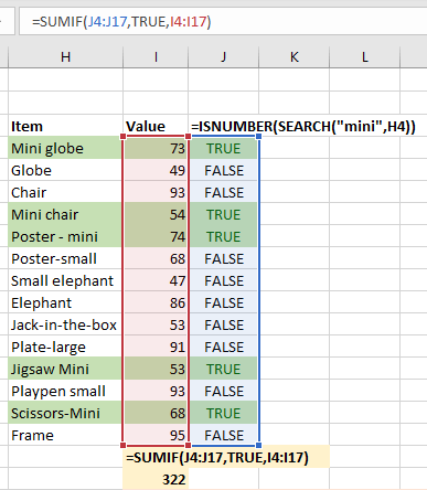 387×444 sum values cells specific text excel excel quick from excelquick.com
  700×400 sum numbers text excel formula exceljet from exceljet.net
  1158×874 excel sum cells text numbers from www.statology.org
  637×127 ms office excel calculate sum values table based from stackoverflow.com
  2530×2475 sum values based criteria column excel from spreadcheaters.com
 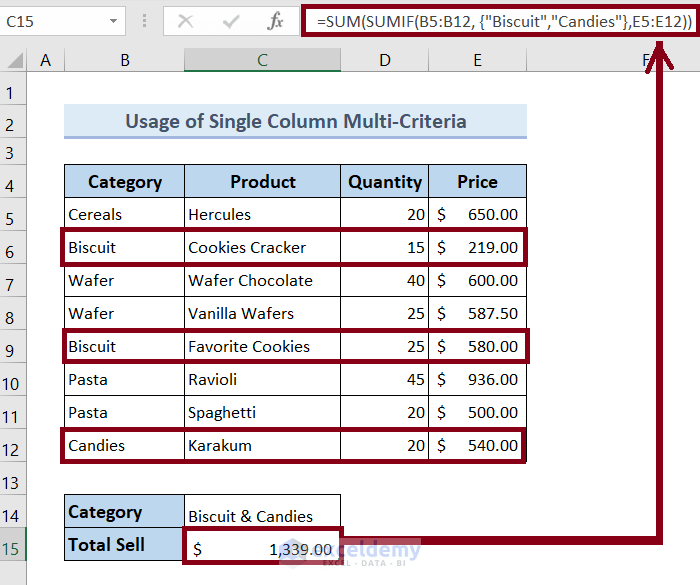 700×585 sum cell text excel suitable examples from www.exceldemy.com
 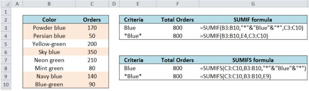 998×295 ways sum cell text excel updf from updf.com
 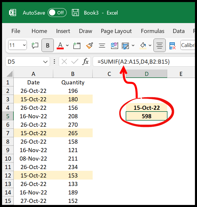 674×709 excel sum values based column header catalog library from catalog.udlvirtual.edu.pe
 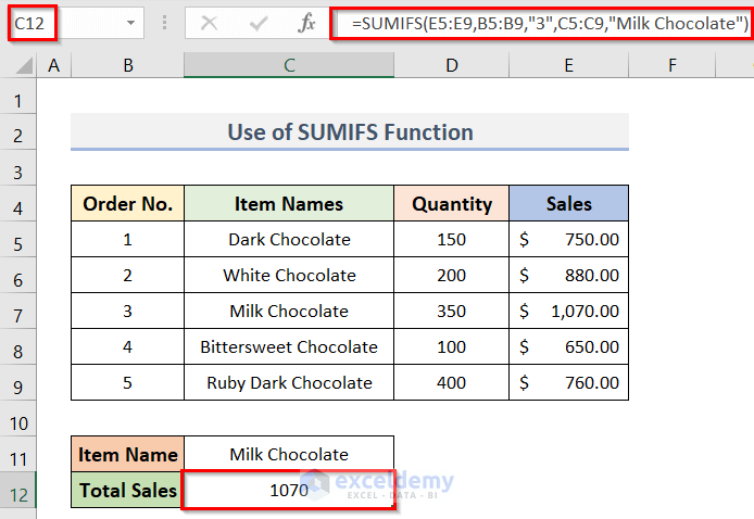 694×478 sum cell text cell excel from www.exceldemy.com
 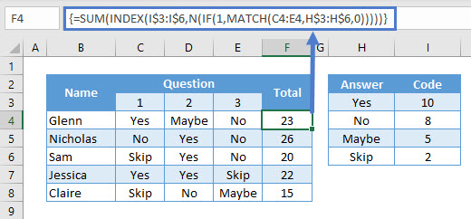 520×242 sum text excel google sheets automate excel from www.automateexcel.com
  767×648 sum cells text numbers excel exceldemy from www.exceldemy.com
  474×270 sum cells specific text excel formula exceljet from exceljet.net
 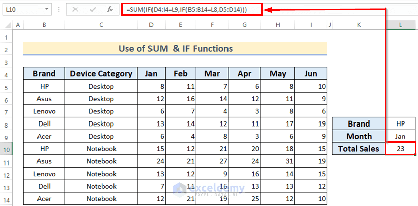 825×407 sum based column row criteria excel ways from www.exceldemy.com
  655×384 sum cells specific text column from www.extendoffice.com
  1280×720 add sum text excel printable templates from read.tupuy.com
  658×356 sum cell number text excel from www.exceldemy.com
  955×287 sum cells text numbers excel from www.extendoffice.com
  872×235 sum values text excel printable templates from read.cholonautas.edu.pe
  700×500 sum cells text numbers excel smart calculations from smartcalculations.com
  1200×630 sum cell text cell excel formula exceljet from exceljet.net
  1280×720 sum specific text excel cells sum cells from www.hotzxgirl.com
  670×307 sum text characters criteria excel from www.exceltip.com
  1280×720 excel sum color subtotal getcell formula earn from earnandexcel.com