How To Do Sensitivity Analysis In Excel
Sensitivity Analysis in Excel
Sensitivity analysis is a crucial technique for understanding how changes in input variables impact the output of a model. In business and finance, it allows you to assess the robustness of your forecasts, investment decisions, and financial models by exploring various scenarios. Excel offers several tools to perform sensitivity analysis, ranging from simple what-if analysis to more sophisticated data tables and scenario management. This guide will walk you through these methods.
1. What-If Analysis: The Foundation
The simplest form of sensitivity analysis in Excel is what-if analysis. This involves manually changing the values of input variables and observing the corresponding changes in the output. While basic, it’s a good starting point to get a feel for how sensitive your model is.
How to Perform What-If Analysis:
- Prepare Your Model: Create your spreadsheet model with clear input variables (e.g., sales growth rate, cost of goods sold) and a calculated output variable (e.g., net profit, return on investment). Ensure the output is linked to the inputs through formulas.
- Identify Key Variables: Determine which input variables are most likely to change or have the greatest impact on the output.
- Manual Adjustment: Simply change the values of your key input variables one at a time. Note the resulting changes in the output variable. For instance, if you’re projecting sales, try increasing and decreasing the sales growth rate by a certain percentage.
- Document the Results: Keep track of the input changes and their corresponding output changes. This documentation helps in understanding the range of possible outcomes.
Example:
Imagine a simple profit calculation:
- Sales Revenue (Input): $100,000
- Cost of Goods Sold (Input): $60,000
- Operating Expenses (Input): $20,000
- Net Profit (Output): = Sales Revenue – Cost of Goods Sold – Operating Expenses = $20,000
You could then test scenarios where sales revenue increases by 10%, decreases by 5%, or where cost of goods sold increases by 2%. Observe how these changes impact the net profit.
Limitations: What-if analysis is tedious and time-consuming for complex models with numerous variables. It also doesn’t provide a structured overview of the sensitivity.
2. Data Tables: A Structured Approach
Data tables provide a more organized way to perform sensitivity analysis by allowing you to systematically vary one or two input variables and observe the impact on a single output variable. This eliminates the need for manually changing inputs repeatedly.
Types of Data Tables:
- One-Variable Data Table: Shows how changes in one input variable affect the output.
- Two-Variable Data Table: Shows how changes in two input variables affect the output.
How to Create a One-Variable Data Table:
- Set up the Input Values: In a column (or row) in your spreadsheet, list the different values you want to test for your input variable. For example, if you want to test sales growth rates from -5% to +5% in 1% increments, list these values in a column.
- Link the Output to the Table: In the cell at the intersection of the row and column of your input values (typically one cell above and to the left of the first input value), enter a formula that refers to the output variable you want to analyze. This is usually a simple `=’cell_with_the_output’` formula.
- Select the Table Range: Select the entire range that includes the input values and the output formula cell.
- Open Data Table: Go to the “Data” tab, click “What-If Analysis,” and then select “Data Table.”
- Specify the Input Cell: In the Data Table dialog box, specify the cell that contains the input variable you are varying. If your input values are in a column, enter the cell reference in the “Column input cell” field. If they are in a row, enter the cell reference in the “Row input cell” field.
- Click OK: Excel will automatically populate the table with the corresponding output values for each input value.
How to Create a Two-Variable Data Table:
- Set up the Input Values: In the first column, list the different values for the first input variable. In the first row, list the different values for the second input variable.
- Link the Output to the Table: In the cell at the intersection of the row and column of your input values (the top-left cell of the data table range), enter a formula that refers to the output variable you want to analyze. This is usually a simple `=’cell_with_the_output’` formula.
- Select the Table Range: Select the entire range that includes both sets of input values and the output formula cell.
- Open Data Table: Go to the “Data” tab, click “What-If Analysis,” and then select “Data Table.”
- Specify the Input Cells: In the Data Table dialog box, enter the cell reference for the first input variable in the “Row input cell” field and the cell reference for the second input variable in the “Column input cell” field.
- Click OK: Excel will populate the table with output values corresponding to each combination of the two input variables.
Example: You might use a two-variable data table to see how varying both sales growth rate and cost of goods sold impact net profit.
3. Scenario Manager: Handling Multiple Scenarios
The Scenario Manager allows you to define and save different sets of input values as “scenarios.” This is useful when you want to analyze distinct possibilities, such as best-case, worst-case, and most-likely scenarios. Unlike data tables, the Scenario Manager can handle multiple input variables simultaneously.
How to Use Scenario Manager:
- Identify Changing Cells: Determine which cells contain the input variables that will change across different scenarios.
- Open Scenario Manager: Go to the “Data” tab, click “What-If Analysis,” and then select “Scenario Manager.”
- Add a Scenario: Click “Add…” to create a new scenario. Give it a descriptive name (e.g., “Best Case,” “Worst Case”).
- Specify Changing Cells: In the “Changing cells” field, enter the cell references of the input variables that will change in this scenario. You can select multiple cells by holding down the Ctrl key while clicking.
- Enter Values: In the next dialog box, enter the values for each changing cell for this particular scenario.
- Repeat for Other Scenarios: Repeat steps 3-5 to create additional scenarios, each with its own set of input values.
- View Scenarios: In the Scenario Manager dialog box, select a scenario and click “Show” to display the results in your spreadsheet.
- Summary Report: You can generate a summary report to compare the output variables across all scenarios. In the Scenario Manager, click “Summary…” and select the cell(s) containing your output variable(s). Choose either a scenario summary or a scenario PivotTable report.
Example: You might create scenarios for “Optimistic,” “Pessimistic,” and “Realistic” sales projections, each with different values for sales growth rate, advertising expenses, and production costs. The scenario manager allows you to easily switch between these scenarios and see the resulting impact on your projected profit.
4. Goal Seek: Working Backwards
Goal Seek allows you to determine what value an input variable needs to be to achieve a specific target value for an output variable. This is essentially reverse sensitivity analysis.
How to Use Goal Seek:
- Select Goal Seek: Go to the “Data” tab, click “What-If Analysis,” and then select “Goal Seek.”
- Set the Parameters:
- Set cell: Enter the cell reference of the output variable you want to target.
- To value: Enter the target value you want the output variable to reach.
- By changing cell: Enter the cell reference of the input variable you want to adjust.
- Click OK: Excel will attempt to find the value for the input variable that achieves the target value for the output variable.
Example: You might use Goal Seek to determine what sales revenue is needed to achieve a net profit of $50,000, given your current cost structure.
Best Practices for Sensitivity Analysis
- Clearly Define Input and Output Variables: Make sure your model is well-structured and easy to understand.
- Document Assumptions: Keep track of the assumptions underlying your model, as these are critical for interpreting the results of your sensitivity analysis.
- Choose Relevant Scenarios: Select scenarios that are realistic and meaningful for your business or investment decisions.
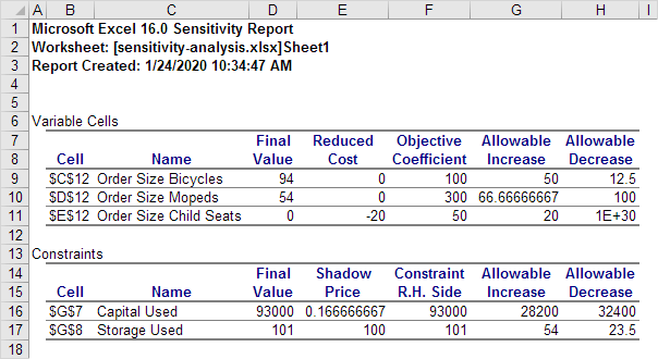
- Use Visualizations: Create charts and graphs to visualize the impact of input variable changes on output variables. This makes it easier to communicate the results of your analysis.
- Consider Correlations: If input variables are correlated, consider the impact of changing them together. Advanced techniques may be needed to analyze correlated variables accurately.
- Understand Limitations: Recognize that sensitivity analysis is only as good as the model it’s based on. A flawed model will produce flawed sensitivity results.
Conclusion
Sensitivity analysis is an essential tool for managing risk and making informed decisions. Excel offers a variety of methods, from simple what-if analysis to more advanced data tables and scenario management, to help you understand how changes in input variables affect the outputs of your models. By utilizing these techniques and following best practices, you can gain valuable insights into the robustness of your forecasts and make more confident choices.
 604×330 sensitivity analysis excel step step tutorial from www.excel-easy.com
  474×277 sensitivity analysis data table excel from www.extendoffice.com
  995×683 excel sensitivity analysis financial modeling class from zica.corporatefinanceinstitute.com
  1298×812 sensitivity analysis excel template sampletemplatess sampletemplatess from www.sampletemplatess.com
 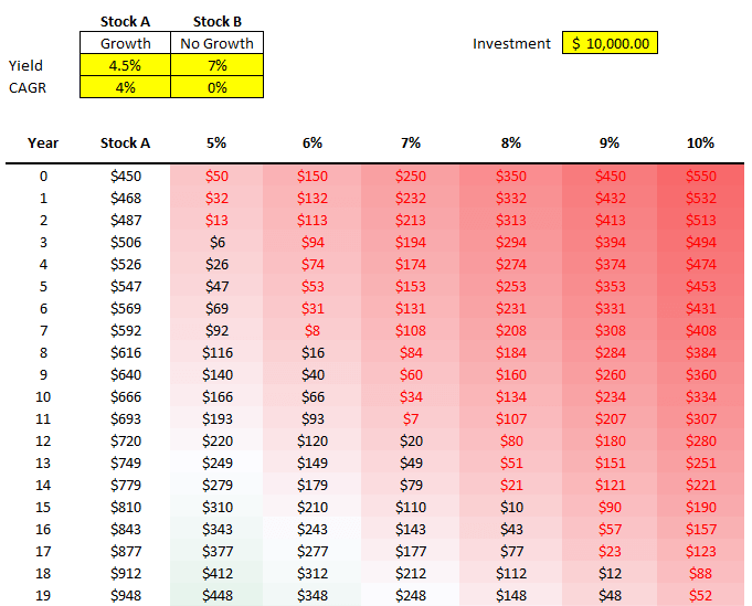 681×549 sensitivity analysis excel howtoexcelnet from howtoexcel.net
  1575×625 sensitivity analysis excel eloquens from www.eloquens.com
  1747×993 sensitivity analysis excel template excel templates excel templates from www.exceltemplate123.us
  914×693 making financial decisions excel sensitivity analysis data from pakaccountants.com