Home » Excel Templates » How To Use Vlookup And Match Together In Excel

How To Use Vlookup And Match Together In Excel

Wednesday, July 16th 2025. | Excel Templates

vlookup partial match excel teachexcelcom

“`html

Combining VLOOKUP and MATCH for Dynamic Excel Lookups

VLOOKUP is a powerful function in Excel for searching a range of cells for a specified value and returning a corresponding value from another column within the same range. However, VLOOKUP has a limitation: it requires you to manually specify the column number from which you want to retrieve the data. This can be cumbersome and prone to errors, especially when the data layout changes or the spreadsheet is large and complex.

This is where the MATCH function comes to the rescue. MATCH searches a range of cells for a specified value and returns the *relative position* of that value within the range. By combining VLOOKUP with MATCH, you can create dynamic lookups that automatically adjust to changes in column positions, making your spreadsheets more flexible and robust.

Understanding VLOOKUP

Before diving into the combination, let’s briefly review the syntax and functionality of VLOOKUP:

=VLOOKUP(lookup_value, table_array, col_index_num, [range_lookup])

lookup_value: The value you want to search for in the first column of the table_array.
table_array: The range of cells that contains the data you want to search. The first column of this range is where the lookup_value is searched.
col_index_num: The column number within the table_array from which you want to retrieve the corresponding value. This is a *fixed number*.
[range_lookup]: An optional argument that specifies whether you want an exact match or an approximate match.
- TRUE or omitted: Approximate match. Requires the first column of table_array to be sorted in ascending order. Returns the largest value less than or equal to lookup_value.
- FALSE: Exact match. Returns the value in the specified column if an exact match for lookup_value is found in the first column of table_array. This is almost always what you want.

The main limitation we want to overcome is the static col_index_num. If the column we need to retrieve data from shifts (e.g., a new column is inserted), the VLOOKUP will return incorrect results until you manually update the col_index_num.

Understanding MATCH

The MATCH function is used to find the position of a value within a range. Here’s the syntax:

=MATCH(lookup_value, lookup_array, [match_type])

lookup_value: The value you want to find in the lookup_array.
lookup_array: The range of cells you want to search. This can be a single row or a single column.
[match_type]: An optional argument that specifies how MATCH searches for the lookup_value.
- 1 or omitted: Finds the largest value that is less than or equal to lookup_value. lookup_array must be sorted in ascending order.
- 0: Finds the first value that is exactly equal to lookup_value. This is generally the safest and most common choice.
- -1: Finds the smallest value that is greater than or equal to lookup_value. lookup_array must be sorted in descending order.

The key takeaway from MATCH is that it returns the *position* of the matching value, not the value itself. This position is a number (e.g., 1, 2, 3), which is exactly what VLOOKUP needs for its col_index_num argument.

Combining VLOOKUP and MATCH

The magic happens when we use MATCH to dynamically determine the col_index_num for VLOOKUP. The general formula structure is:

=VLOOKUP(lookup_value, table_array, MATCH(column_header, header_row, 0), FALSE)

Let’s break this down:

lookup_value: The same as in a regular VLOOKUP – the value you are searching for.
table_array: The same as in a regular VLOOKUP – the range containing the data.
MATCH(column_header, header_row, 0): This part replaces the static col_index_num.
- column_header: The header of the column you want to retrieve data from. This is the value MATCH will search for.
- header_row: The row containing the column headers. This is where MATCH will search for column_header.
- 0: Specifies an exact match for column_header.
This MATCH function will return the column number where the column_header is found within the header_row.
FALSE: Specifies an exact match for the lookup_value in the first column of the table_array. This is crucial for accurate lookups.

Example Scenario

Imagine you have a table of employee data in an Excel sheet. The columns are: Employee ID, Name, Department, Salary, and Hire Date. You want to look up an employee by their Employee ID and retrieve their Salary. However, the order of the columns might change in the future. Here’s how you can use VLOOKUP and MATCH together to ensure your formula still works even if the column order changes:

**Data Table:** Assume your data is in the range A1:E100. Row 1 contains the column headers.
**Lookup Value:** Let’s say you have the Employee ID you want to look up in cell G2.
**Column Header:** The header for the Salary column is “Salary”. You can either type this directly into the formula, or reference a cell (e.g., H2) containing the text “Salary”. Referencing a cell is generally better for readability and maintainability.
**Header Row:** The header row is A1:E1.

The formula would be:

=VLOOKUP(G2, A1:E100, MATCH(H2, A1:E1, 0), FALSE)

In this formula:

G2 is the lookup_value (Employee ID).
A1:E100 is the table_array.
MATCH(H2, A1:E1, 0) finds the column number of the “Salary” column (assuming “Salary” is in cell H2) within the header row A1:E1. If “Salary” is in the 4th column, MATCH will return 4.
FALSE ensures an exact match for the Employee ID.

If the “Salary” column moves to a different position (e.g., becomes the 3rd column), the MATCH function will automatically adjust and return the correct column number. The VLOOKUP will then retrieve the Salary from the correct column, without requiring any manual updates to the formula.

Benefits of Using VLOOKUP and MATCH Together

**Flexibility:** Adapts automatically to changes in column positions.
**Robustness:** Less prone to errors caused by data rearrangement.
**Maintainability:** Easier to understand and update compared to formulas with hardcoded column numbers.
**Dynamic Reporting:** Enables creating dynamic reports where column selections can be easily changed using dropdown menus or other controls, affecting which data is retrieved by the VLOOKUP.

Important Considerations

**Exact Matches:** Always use FALSE for the range_lookup argument in VLOOKUP and 0 for the match_type argument in MATCH unless you have a specific reason to use approximate matching. Using exact matches ensures that you’re retrieving the correct data.
**Header Row Consistency:** Ensure that the values in the header row (header_row) exactly match the column_header you’re searching for. Even a small difference in spelling or spacing will cause MATCH to fail.
**Error Handling:** Consider using IFERROR to handle cases where the lookup_value is not found in the table or the column_header is not found in the header row. This can prevent unsightly error messages and provide more informative feedback to the user. For example: =IFERROR(VLOOKUP(G2, A1:E100, MATCH(H2, A1:E1, 0), FALSE), "Value Not Found").
**Performance:** For very large datasets, using INDEX and MATCH might offer better performance than VLOOKUP. However, for most common scenarios, the performance difference is negligible.

Conclusion

Combining VLOOKUP and MATCH is a powerful technique that significantly enhances the flexibility and robustness of your Excel spreadsheets. By dynamically determining the column number using MATCH, you can create formulas that automatically adapt to changes in data layout, reducing the risk of errors and making your spreadsheets easier to maintain. This combination is a valuable skill for anyone working with data in Excel, especially when dealing with complex or frequently changing datasets.

“`

650×421 vlookup partial match excel teachexcelcom from www.teachexcel.com

590×380 vlookup match quadexcelcom from quadexcel.com

704×350 vlookup match tables excelnotes from excelnotes.com

609×369 vlookup match dynamic duo excel campus from www.excelcampus.com

1280×720 vlookup approximate match microsoft excel basic advanced from www.goskills.com

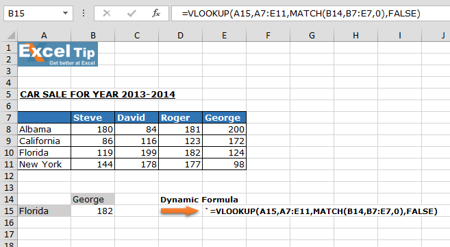657×360 vlookup match formulas excel from www.exceltip.com

Post Views: 77