How To Use Randbetween Function In Excel For Simulation
“`html
Using RANDBETWEEN for Simulation in Excel
The RANDBETWEEN function in Excel is a powerful tool for creating simulations. It allows you to generate random integers within a specified range, which can be used to model various scenarios, perform Monte Carlo simulations, and analyze probabilities. This guide will walk you through the basics of RANDBETWEEN and demonstrate how to use it effectively for simulation purposes, illustrated with various examples.
Understanding the RANDBETWEEN Function
The RANDBETWEEN function takes two arguments:
- bottom: The smallest integer that
RANDBETWEENwill return. - top: The largest integer that
RANDBETWEENwill return.
The syntax is simple: =RANDBETWEEN(bottom, top)
Each time the worksheet is calculated (by pressing F9, changing a cell value, or automatically), RANDBETWEEN generates a new random integer within the specified range. This dynamic nature is crucial for simulation. Importantly, RANDBETWEEN only generates integers, not decimals. If you need decimal values, you can combine it with division or other mathematical operations.
Basic Simulation Examples
1. Simulating a Coin Flip
To simulate a coin flip (heads or tails), we can assign 1 to heads and 0 to tails (or vice-versa). The RANDBETWEEN function allows us to generate either 0 or 1 randomly.
- In cell A1, enter the formula:
=RANDBETWEEN(0,1) - Each time you recalculate the sheet (press F9), cell A1 will display either 0 or 1, representing the outcome of a coin flip.
- To interpret the results, you can use an
IFstatement in cell B1:=IF(A1=0,"Tails","Heads").
2. Simulating a Dice Roll
To simulate rolling a six-sided die, we need a random integer between 1 and 6.
- In cell A1, enter the formula:
=RANDBETWEEN(1,6) - Each time you recalculate the sheet, cell A1 will display a random number between 1 and 6, simulating a dice roll.
3. Simulating a Deck of Cards (Basic)
Let’s say we want to draw a card from a deck and assign a number to each card (ignoring suits for simplicity): Ace=1, 2=2,… 10=10, Jack=11, Queen=12, King=13.
- In cell A1, enter the formula:
=RANDBETWEEN(1,13) - To display the card name instead of the number, use a
CHOOSEfunction in cell B1:=CHOOSE(A1,"Ace","2","3","4","5","6","7","8","9","10","Jack","Queen","King")
More Advanced Simulations
1. Monte Carlo Simulation for Project Management
Let’s simulate the completion time for a project that has three tasks, each with uncertain durations.
Assumptions:
- Task 1: Duration between 5 and 10 days
- Task 2: Duration between 7 and 12 days
- Task 3: Duration between 3 and 8 days
- In cell A1, enter “Task 1 Duration”:
=RANDBETWEEN(5,10) - In cell A2, enter “Task 2 Duration”:
=RANDBETWEEN(7,12) - In cell A3, enter “Task 3 Duration”:
=RANDBETWEEN(3,8) - In cell A4, enter “Total Duration”:
=SUM(A1:A3)
Now, to perform a Monte Carlo simulation, you need to repeat this calculation multiple times and record the total duration. Since manually recalculating and recording values would be tedious, we use the Data Table feature in Excel.
- In a separate column (e.g., Column C), enter a list of numbers from 1 to, say, 1000 (representing 1000 simulations). You can do this quickly by entering 1 in C1, 2 in C2, and then dragging the fill handle down to C1000.
- In cell D1, enter the formula:
=A4(this links cell D1 to the total duration calculation). - Select the range C1:D1000.
- Go to the Data tab, click What-If Analysis, and choose Data Table.
- In the Data Table dialog box, leave the Row input cell blank.
- In the Column input cell, enter any empty cell outside of your data range (e.g., E1). Excel will use this empty cell to trick the formulas in A1:A3 into recalculating.
- Click OK.
Now, Column D contains 1000 different total durations based on random durations for the three tasks. You can analyze this data to estimate the probability of completing the project within a certain timeframe. For example, you can use the COUNTIF function to count how many times the total duration is less than 25 days: =COUNTIF(D1:D1000,"<25")/1000 (this gives you the probability as a decimal). You can then use AVERAGE, MAX, MIN, and STDEV.S to get descriptive statistics of your simulated project durations.
2. Inventory Simulation
Let's simulate an inventory system to determine the optimal order quantity.
Assumptions:
- Daily demand follows a uniform distribution between 10 and 30 units.
- Lead time (time to receive an order) is between 2 and 5 days.
- We want to determine the reorder point (when to place an order) and order quantity to minimize stockouts.
Set up the following columns:
- A: Day (Enter numbers 1, 2, 3... down to, say, 365 for a year)
- B: Demand:
=RANDBETWEEN(10,30) - C: On Hand: Initial inventory level (e.g., 100). For subsequent days,
=MAX(0, previous day's On Hand - previous day's Demand + units received today) - D: Order Placed?:
=IF(C2 < Reorder Point, 1, 0). The `Reorder Point` will be a cell you can adjust to see the impact. You'll need to define this cell outside the data table (e.g., F1) and refer to it using an absolute reference: `IF(C2 < $F$1, 1, 0)` - E: Lead Time: If an order is placed today, generate the lead time:
=IF(D2=1,RANDBETWEEN(2,5),0) - F: Units Ordered: If an order is placed today, generate the order quantity:
=IF(D2=1, Order Quantity, 0). The `Order Quantity` will also be a cell you can adjust (e.g., G1) and should be referred to with an absolute reference: `IF(D2=1,$G$1,0)` - G: Units Received Today: Check if an order placed "Lead Time" days ago is delivered today. This requires a more complex formula and referencing previous rows. For example, for row 6: `=IF(SUMIFS($F$2:F5,$E$2:E5,4)=0,0,SUMIFS($F$2:F5,$E$2:E5,4))` This means 'If the sum of "Units Ordered" for orders with a lead time of 4 days ending *yesterday* is 0, then 0 units are received. Otherwise, units equal to the sum of previous orders with a lead time of 4 days are received. The '4' needs to decrement depending on the row.
This model is more complex and requires careful referencing of cells. You will also need to handle the initial few days (where lead times may refer to days before the start of the simulation) appropriately. You would then create a Data Table to iterate through different Reorder Point and Order Quantity values (using a two-variable data table) and calculate the number of stockouts (days where On Hand is 0) for each combination.
Important Considerations
- Recalculation: Remember that
RANDBETWEENrecalculates every time the worksheet changes. This is essential for the simulation. - Seed Values: By default, Excel uses a pseudo-random number generator. While generally sufficient, you might consider using add-ins for more sophisticated random number generation or controlling the seed value for reproducibility in specific scenarios.
- Data Table Limitations: The Data Table feature can be slow with very large datasets. For more complex simulations with a large number of iterations, consider using VBA (Visual Basic for Applications) or a dedicated simulation tool.
- Model Validation: Always validate your simulation model by comparing the results to real-world data or theoretical expectations, if possible. This ensures the model is reasonably accurate and useful.
- Understanding Distributions:
RANDBETWEENgenerates a *uniform* distribution. If your data follows a different distribution (e.g., normal distribution), you may need to use other Excel functions or methods to simulate that distribution. For example, you could useNORM.INV(RAND(), mean, standard_deviation)for a normal distribution.
By understanding the RANDBETWEEN function and applying it creatively, you can build a wide variety of simulations in Excel to model complex systems, analyze risks, and make better decisions.
```
 752×551 excel randbetween function video from trumpexcel.com
  1200×684 randbetween function excelnotes from excelnotes.com
 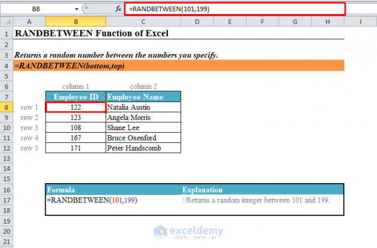 768×505 randbetween function excel examples exceldemy from www.exceldemy.com
  768×535 calculate random integers randbetween function from gyankosh.net
  700×415 randbetween function excel from www.thewindowsclub.com