How To Use COUNTIFS With Multiple Conditions In Excel
Using COUNTIFS with Multiple Conditions in Excel
The COUNTIFS function in Excel is a powerful tool for counting cells that meet multiple criteria. Unlike its predecessor, COUNTIF, which can only handle a single condition, COUNTIFS allows you to specify numerous conditions across different ranges, making it incredibly versatile for data analysis.
Understanding the Syntax
The syntax of the COUNTIFS function is as follows:
COUNTIFS(criteria_range1, criteria1, [criteria_range2, criteria2], ...)
criteria_range1: The first range of cells to evaluate. This is a mandatory argument.criteria1: The criterion to apply tocriteria_range1. This is also a mandatory argument.[criteria_range2, criteria2]: Optional. Additional ranges and their associated criteria. You can add up to 127 range/criteria pairs.
The function returns the number of cells that meet all specified conditions. It’s important to remember that COUNTIFS uses an “AND” logic – a cell must satisfy every criterion to be counted.
Basic Examples
Let’s start with some simple examples to illustrate the basic usage of COUNTIFS.
Imagine you have a table of sales data with columns for “Region,” “Product,” and “Sales Amount.”
| Region | Product | Sales Amount |
|---|---|---|
| North | Widget A | 150 |
| South | Widget B | 200 |
| North | Widget B | 180 |
| East | Widget A | 120 |
| North | Widget A | 220 |
| South | Widget A | 250 |
Suppose you want to count the number of sales records where the “Region” is “North” and the “Product” is “Widget A.” You could use the following formula:
=COUNTIFS(A2:A7, "North", B2:B7, "Widget A")
In this formula:
A2:A7is the range containing the “Region” data."North"is the criterion for the “Region” column.B2:B7is the range containing the “Product” data."Widget A"is the criterion for the “Product” column.
The formula will return `2` because there are two records that meet both conditions.
Now, let’s say you want to count the number of sales records where the “Region” is “South” and the “Sales Amount” is greater than 200. The formula would be:
=COUNTIFS(A2:A7, "South", C2:C7, ">200")
Here, ">200" is the criterion for the “Sales Amount” column. It uses a comparison operator to specify that the value must be greater than 200. This formula will return `1`.
Using Cell References
Instead of hardcoding the criteria directly into the formula, you can use cell references. This makes your formulas more dynamic and easier to update. For example, if you have the region “North” in cell E1 and the product “Widget A” in cell E2, the formula would become:
=COUNTIFS(A2:A7, E1, B2:B7, E2)
If you change the value in cell E1 to “South,” the formula will automatically recalculate based on the new region.
Using Wildcards
COUNTIFS supports the use of wildcard characters: * (asterisk) and ? (question mark).
*represents zero or more characters.?represents a single character.
For instance, to count the number of products that start with “Widget,” you can use the following formula (assuming the product names are in column B):
=COUNTIFS(B2:B7, "Widget*")
This will count “Widget A,” “Widget B,” and any other product names starting with “Widget.”
To count the number of products that are exactly six characters long and start with “W,” you could use:
=COUNTIFS(B2:B7, "W?????")
Using Dates
COUNTIFS can also be used with dates. Suppose you have a column (D) with dates, and you want to count the number of entries within a specific date range. Let’s say you want to count the entries between January 1, 2023, and January 31, 2023. You can use the DATE function to create the date criteria:
=COUNTIFS(D2:D10, ">="&DATE(2023,1,1), D2:D10, "<="&DATE(2023,1,31))
The DATE(year, month, day) function returns a date value. The & operator is used to concatenate the comparison operator (">=" or "<=") with the date value.
Alternatively, you can reference cells containing the start and end dates. If cell F1 contains the start date and cell F2 contains the end date, the formula would be:
=COUNTIFS(D2:D10, ">="&F1, D2:D10, "<="&F2)
Important Considerations and Potential Errors
- Case Sensitivity:
COUNTIFSis generally not case-sensitive. "North" is usually treated the same as "north." However, this can depend on your Excel settings and regional settings. - Data Types: Ensure that the data in your criteria range matches the data type of your criteria. Trying to compare text to a number directly can lead to unexpected results.
- Ranges Must Be the Same Size: All
criteria_rangearguments must have the same number of rows and columns. If the ranges are different sizes,COUNTIFSwill return a#VALUE!error. - Empty Cells: Empty cells are generally treated as zero for numerical comparisons and as empty strings for text comparisons. Be aware of how empty cells might affect your counts.
- Quotation Marks: Text criteria and criteria containing comparison operators must be enclosed in double quotation marks. Numerical criteria that are directly entered (not part of a comparison) do not need quotation marks. For example,
100does not need quotes, but">100"does. - Formula Errors: Double-check your formula for typos, missing commas, or incorrect cell references. Use Excel's formula auditing tools to help identify and correct errors.
Advanced Examples
Let's look at a more complex example. Suppose you want to count the number of sales records where:
- The "Region" is either "North" or "South."
- The "Product" is "Widget A."
- The "Sales Amount" is greater than 150.
Unfortunately, COUNTIFS doesn't directly support "OR" logic within a single criterion range. To achieve this, you can use a combination of COUNTIFS and SUM:
=SUM(COUNTIFS(A2:A7, {"North","South"}, B2:B7, "Widget A", C2:C7, ">150"))
In this formula:
{"North","South"}creates an array of two criteria for the "Region" column.COUNTIFSis calculated twice, once for "North" and once for "South" (along with the other conditions).SUMadds the results of the twoCOUNTIFScalculations, effectively implementing the "OR" logic for the region.
This formula will return the number of sales records that meet the combined criteria.
Another approach to handling more complex logic is to create helper columns. For example, you could create a helper column that contains a flag (e.g., TRUE/FALSE) indicating whether a row meets a specific set of conditions. You can then use a simpler COUNTIF or COUNTIFS on the helper column.
Conclusion
COUNTIFS is a powerful and flexible function for counting cells based on multiple conditions in Excel. By understanding its syntax, using cell references, wildcards, and date functions, and being aware of potential errors, you can effectively analyze your data and extract valuable insights. Remember to consider using SUM and helper columns for more complex logical conditions.
 474×221 excel countif multiple criteria alert data from alert.mc.edu
  669×631 excel countif multiple criteria gaseled from gaseled.weebly.com
  847×594 countifs multiple conditions columns excel from stackoverflow.com
 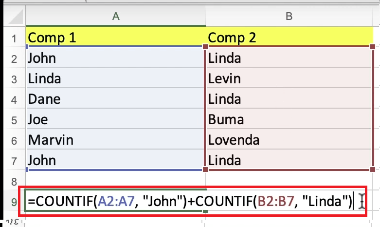 781×466 countif function excel multiple criteria andor exceltutorial from www.exceltutorial.net
  1106×700 countif excel multiple criteria couplerio blog from blog.coupler.io
  661×366 excel countif multiple criteria snoclock from snoclock.weebly.com
 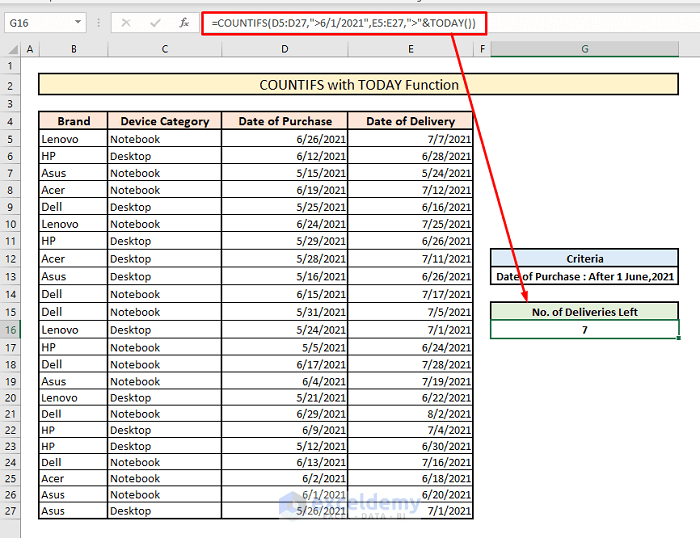 700×538 countifs count multiple columns excel exceldemy from www.exceldemy.com
  570×362 countif multiple criteria guide countifs excel from corporatefinanceinstitute.com
 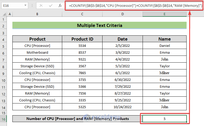 774×481 apply countif function excel multiple criteria from www.exceldemy.com
  414×203 trending formula excel multiple conditions latest from www.hotzxgirl.com
  300×195 countif multiple criteria excel formula from www.excelmojo.com
  662×380 countif multiple criteria excel from www.extendoffice.com
 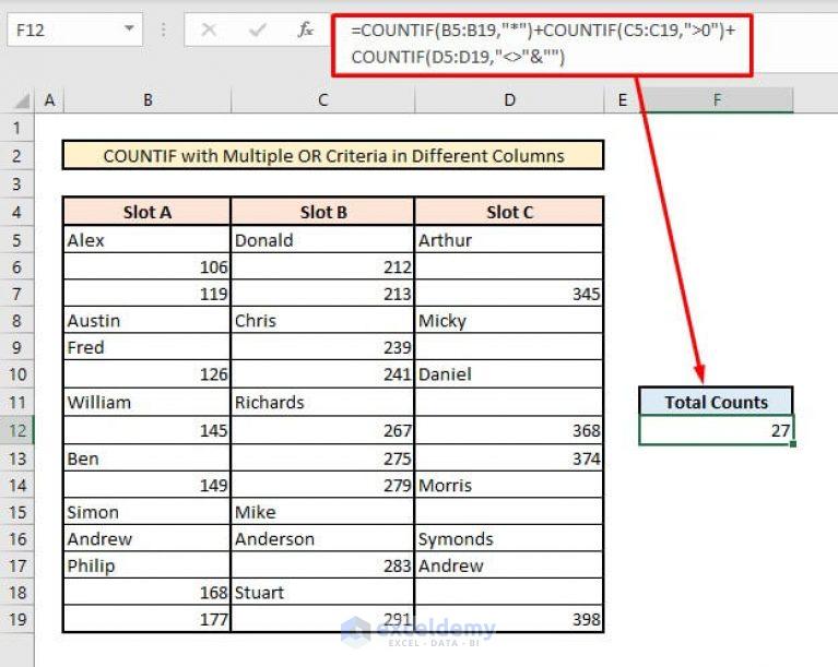 767×611 countif multiple criteria columns excel exceldemy from www.exceldemy.com
  700×313 countif multiple criteria countifs excel from fundsnetservices.com
  1280×720 countif multiple criteria countif function earn excel from earnandexcel.com
 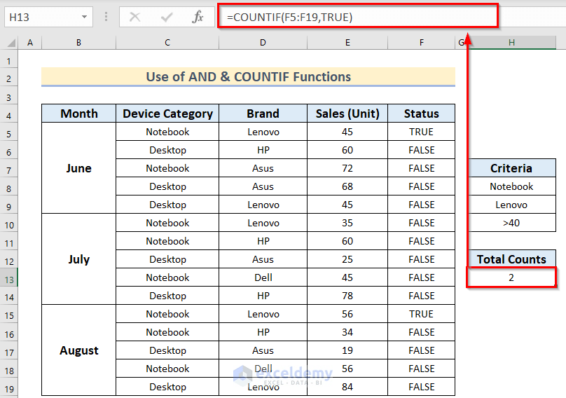 808×568 countif multiple criteria columns excel from www.exceldemy.com
 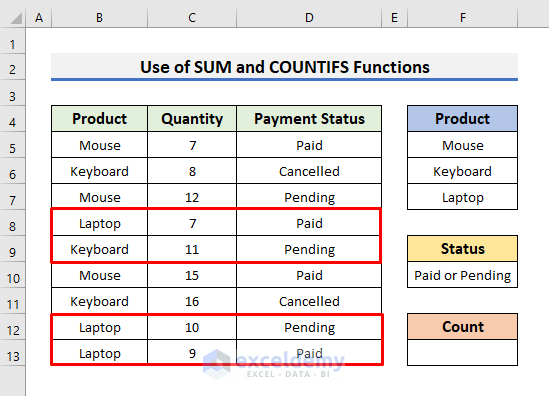 549×396 excel countifs function multiple criteria from www.exceldemy.com
  700×400 countifs multiple criteria logic excel formula exceljet from exceljet.net
  531×306 countif multiple criteria excel tutorial riset from riset.guru
  1280×720 work excel sheet multiple users lioneon from lioneon.weebly.com
  1280×720 excel easy countif multiple criteria myexcelonline from www.myexcelonline.com
  1280×720 countif function excel multiple ranges from web.australiahealthy.com
  527×281 excel mac count conditions columns zoomfoot from zoomfoot.weebly.com
  1024×627 excel countifs count cells multiple criteria from thatexcelsite.com