How To Use Conditional Formatting With Formulas In Excel
Here’s a comprehensive guide on using conditional formatting with formulas in Excel, formatted as requested:
Excel’s conditional formatting is a powerful tool for highlighting cells based on specific criteria. While simple rules can highlight values greater than, less than, or equal to a certain number, the real magic happens when you use formulas to define the formatting conditions. This allows for complex, dynamic, and highly customized highlighting based on relationships between cells, text patterns, dates, and more.
Understanding the Basics
Before diving into formulas, it’s important to understand the fundamental steps for applying conditional formatting:
- Select the Range: First, select the cells you want to apply the conditional formatting to. This is crucial, as the formula you write will be evaluated relative to the top-left cell of this selected range.
- Access Conditional Formatting: Go to the “Home” tab on the Excel ribbon, then click “Conditional Formatting.”
- Choose “New Rule…”: From the dropdown menu, select “New Rule…”
- Select “Use a formula to determine which cells to format”: In the “New Formatting Rule” dialog box, choose the option “Use a formula to determine which cells to format.” This is where you’ll enter your formula.
- Enter the Formula: Enter your formula in the provided text box. The formula must evaluate to either TRUE or FALSE. If the formula returns TRUE for a specific cell in the selected range (based on the formula’s evaluation relative to the top-left cell), that cell will be formatted.
- Set the Format: Click the “Format…” button to choose the desired formatting (e.g., font color, background color, border, etc.).
- Click OK: Click “OK” on both the “Format Cells” dialog and the “New Formatting Rule” dialog to apply the rule.
Key Concepts for Formulas in Conditional Formatting
These concepts are essential for writing effective conditional formatting formulas:
- Relative vs. Absolute References: Understanding cell references is critical. A relative reference (e.g., A1) changes based on the cell being evaluated. An absolute reference (e.g., $A$1) always refers to the same cell, regardless of which cell is being evaluated. A mixed reference (e.g., $A1 or A$1) locks either the column or the row, respectively. When writing a formula for conditional formatting, always think about which parts of the formula should remain constant and which parts should change as the formula is applied to different cells in the selected range. The top-left cell of your selected range will be considered the ‘active’ cell for Excel to calculate the formula.
- Boolean Logic: Conditional formatting formulas rely on Boolean logic – TRUE or FALSE. The formula must return TRUE for the cell to be formatted. You’ll use comparison operators (>, <, =, >=, <=, <>) and logical functions (AND, OR, NOT) to create these conditions.
- Formulas Relative to the Top-Left Cell: The formula is always evaluated relative to the top-left cell of the selected range. For example, if you select the range B2:D10 and the formula is `=A2>10`, Excel will interpret this as “Is the value in the cell to the left of the current cell greater than 10?” for each cell in the range B2:D10.
- Order of Operations: Remember the order of operations (PEMDAS/BODMAS). Use parentheses to control the order in which Excel evaluates your formula.
Examples of Conditional Formatting Formulas
Here are several examples demonstrating how to use formulas for conditional formatting:
1. Highlighting Duplicate Values in a Column
To highlight duplicate entries in column A:
- Select column A.
- Create a new rule using a formula.
- Enter the following formula: `=COUNTIF($A:$A,A1)>1`
- Set the desired formatting.
Explanation:
- `COUNTIF($A:$A,A1)`: This counts the number of times the value in cell A1 appears in the entire column A. The `$A:$A` makes the column absolute, so the count always refers to the entire column. `A1` is relative, so as the formatting is applied to other cells in column A, it checks the count for each cell’s respective value.
- `>1`: This checks if the count is greater than 1, indicating that the value appears more than once (i.e., it’s a duplicate).
2. Highlighting Rows Based on a Cell Value in a Specific Column
To highlight the entire row if the value in column C is “Complete”:
- Select the entire data range (e.g., A1:E10).
- Create a new rule using a formula.
- Enter the following formula: `=$C1=”Complete”`
- Set the desired formatting.
Explanation:
- `$C1`: This locks the column to C (using `$C`) but keeps the row relative (using `1`). This ensures that the formula always checks the value in column C for each row, but it checks a different row for each row being formatted.
- `=”Complete”`: This compares the value in column C to the text “Complete”.
3. Highlighting Cells Based on a Date Range
To highlight dates within the next 7 days in column B:
- Select column B.
- Create a new rule using a formula.
- Enter the following formula: `=AND(B1>=TODAY(),B1<=TODAY()+7)`
- Set the desired formatting.
Explanation:
- `TODAY()`: This function returns the current date.
- `TODAY()+7`: This calculates the date 7 days from today.
- `AND(B1>=TODAY(),B1<=TODAY()+7)`: The `AND` function ensures that both conditions are true: the date in cell B1 must be greater than or equal to today's date *and* less than or equal to the date 7 days from today.
4. Highlighting Cells Based on a Numerical Range with a Lower and Upper Bound
To highlight cells in column D if they fall between 50 and 100 (inclusive):
- Select column D.
- Create a new rule using a formula.
- Enter the following formula: `=AND(D1>=50, D1<=100)`
- Set the desired formatting.
Explanation:
- `AND(D1>=50, D1<=100)`: The `AND` function requires both conditions to be TRUE for a cell to be highlighted. `D1>=50` checks if the value in cell D1 is greater than or equal to 50. `D1<=100` checks if the value in cell D1 is less than or equal to 100.
5. Highlighting Cells Based on a Value in Another Sheet
To highlight cells in Sheet1!Column A if their values are present in Sheet2!Column B:
- Select Sheet1!Column A.
- Create a new rule using a formula.
- Enter the following formula: `=NOT(ISERROR(MATCH(A1,Sheet2!$B:$B,0)))`
- Set the desired formatting.
Explanation:
- `MATCH(A1,Sheet2!$B:$B,0)`: This searches for the value of A1 within Sheet2!Column B. The `$B:$B` makes the column absolute. The `0` argument specifies an exact match. If a match is found, it returns the position of the match; otherwise, it returns an error (#N/A).
- `ISERROR(…)`: This checks if the result of the MATCH function is an error. It returns TRUE if there’s an error (no match found) and FALSE if a match is found.
- `NOT(…)`: This inverts the result of ISERROR. So, it returns TRUE if a match is found (no error) and FALSE if no match is found (error). Therefore, only values present in Sheet2!Column B will be highlighted in Sheet1!Column A.
6. Highlighting every other row
- Select the entire data range.
- Create a new rule using a formula.
- Enter the following formula: `=MOD(ROW(),2)=0`
- Set the desired formatting.
Explanation
- `ROW()`: Returns the row number of the cell.
- `MOD(ROW(),2)`: Returns the remainder after dividing the row number by 2.
- `=0`: Checks if the remainder is 0. Even rows will have a remainder of 0 when divided by 2.
To highlight odd rows instead, use the formula `=MOD(ROW(),2)=1`
Tips and Troubleshooting
- Test Your Formulas: Before applying conditional formatting, test your formula in a cell within your spreadsheet to ensure it returns TRUE or FALSE as expected. This helps you debug your logic before committing to the formatting rule.
- Use the Formula Auditing Tools: Excel’s “Evaluate Formula” tool (under the “Formulas” tab) can be helpful for stepping through complex formulas and understanding how they are being evaluated.
- Manage Rules: Use the “Conditional Formatting” -> “Manage Rules…” option to edit, delete, reorder, or see all conditional formatting rules applied to a worksheet. Rule order matters; the first rule that evaluates to TRUE will be applied, and subsequent rules may be ignored.
- Formula Errors: Double-check your formula for syntax errors, incorrect cell references, and mismatched parentheses. Excel’s error messages can provide clues, but sometimes it’s best to start fresh.
- Performance: Excessive use of conditional formatting, especially with complex formulas, can slow down Excel. Try to optimize your formulas and avoid applying conditional formatting to excessively large ranges unless absolutely necessary.
- Locked sheets: When the sheet is locked and conditional formatting is not working, check if the “Format Cells” option is selected in the “Allow users to edit ranges” dialog.
Conditional formatting with formulas is a powerful way to visualize data and gain insights in Excel. By mastering the concepts of relative and absolute references, Boolean logic, and the nuances of formula evaluation, you can create highly customized and dynamic highlighting rules to make your spreadsheets more informative and effective.
 882×508 conditional formulas conditional formatting excel quadexcelcom from quadexcel.com
 :max_bytes(150000):strip_icc()/ExcelConditionalFormattingNewRule-5c57373f4cedfd0001efe4d4.jpg) 1596×882 formulas conditional formatting excel from www.lifewire.com
1596×882 formulas conditional formatting excel from www.lifewire.com  450×450 conditional formatting formulas excel from professor-excel.com
  700×400 excel conditional formatting formulas from www.micoope.com.gt
  473×461 ms excel conditional formatting formulas riset from riset.guru
  700×400 conditional formatting based cell excel formula exceljet from exceljet.net
  865×628 excel conditional formatting compumzaer from compumzaer.weebly.com
  800×600 excel conditional formatting formula customguide from www.customguide.com
  800×600 excel conditional formatting customguide from www.customguide.com
  966×722 conditional formatting excel formulas riset from riset.guru
 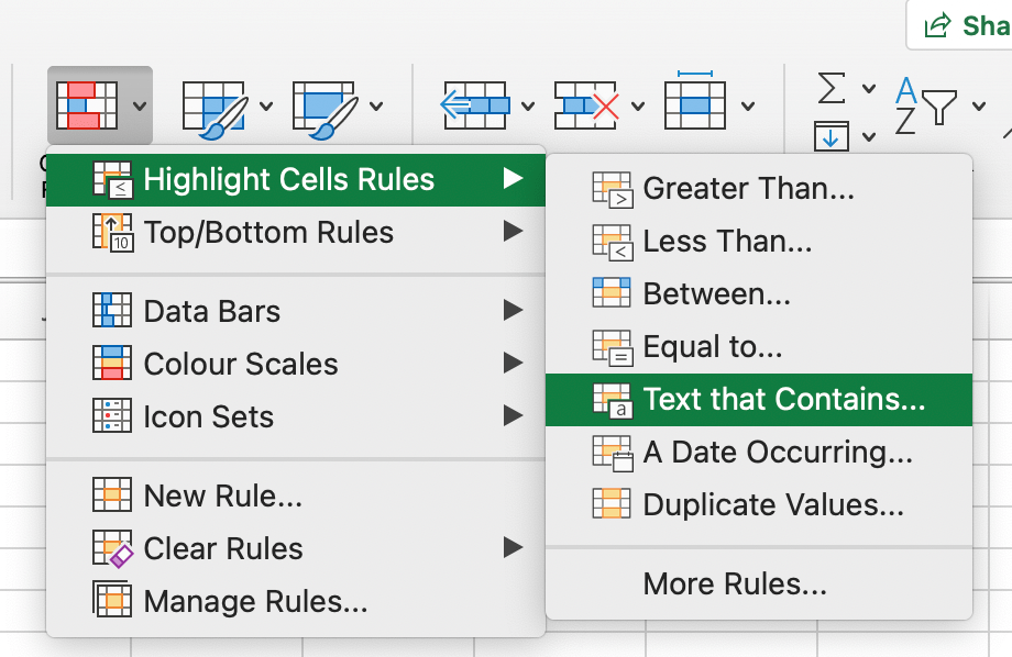 920×598 conditional formatting excel smart calculations from smartcalculations.com
  681×541 conditional formatting excel beginners guide from www.goskills.com
  622×378 understanding excel conditional formatting formula from www.projectcubicle.com
  555×458 conditional formatting formulas excel vrogueco from www.vrogue.co
  642×530 excel conditional formatting formulas based cell from www.ablebits.com
  1024×557 conditional formatting dataliticocom from datalitico.com
  1920×1080 conditional formatting excel business computer skills from www.businesscomputerskills.com
 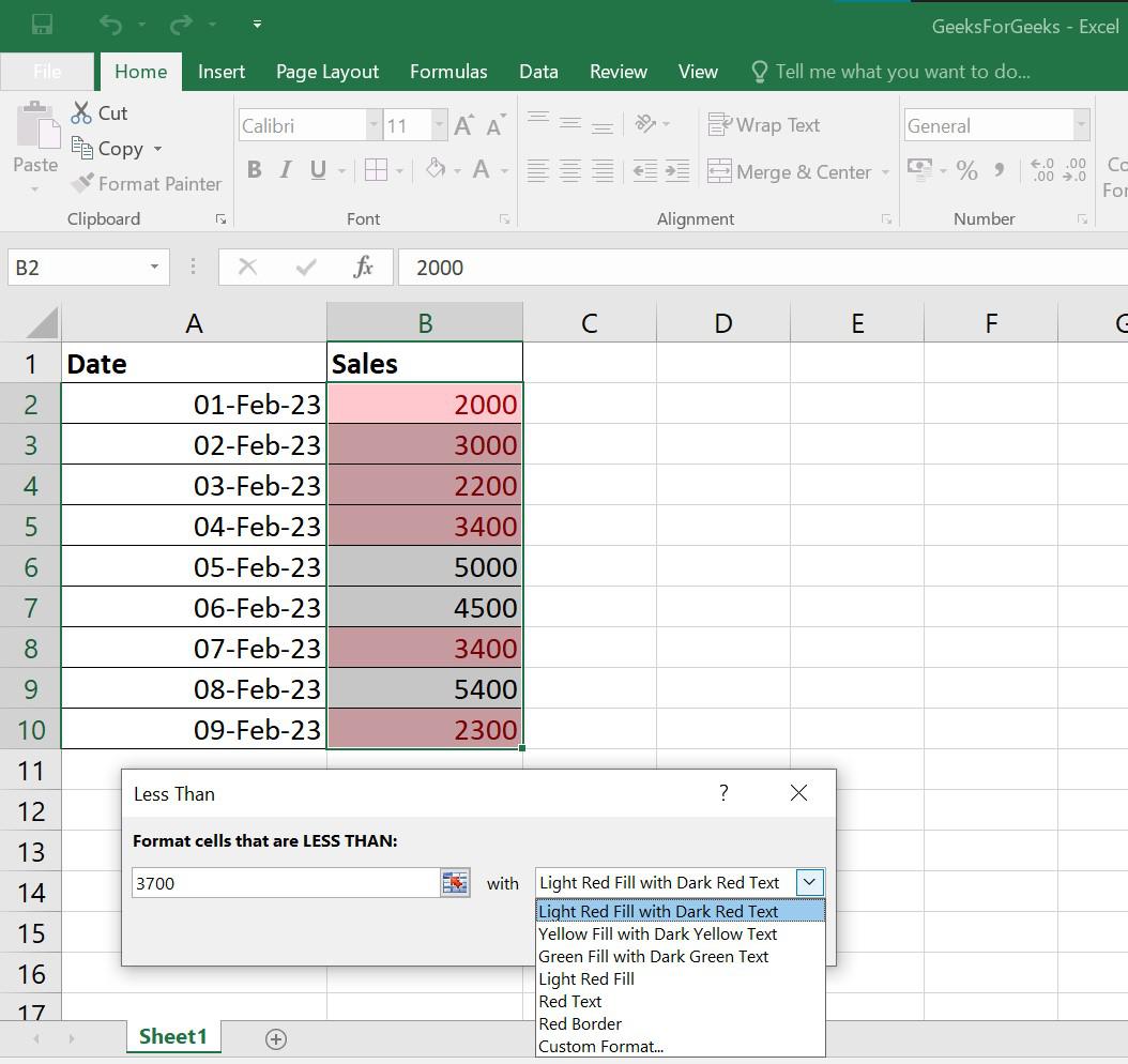 1054×994 excel conditional formatting examples geeksforgeeks from www.geeksforgeeks.org
  1200×630 formula conditional formatting video exceljet from exceljet.net
  500×290 perform conditional formatting formula excel from www.exceltip.com
  982×615 conditional formatting excel from www.geeksforgeeks.org
  1076×424 conditional formatting based formula excel google sheets from www.automateexcel.com
  720×844 conditional formatting excel geeksforgeeks from www.geeksforgeeks.org
  768×620 conditional formatting excel cell text formula from www.howtoexcelatexcel.com
 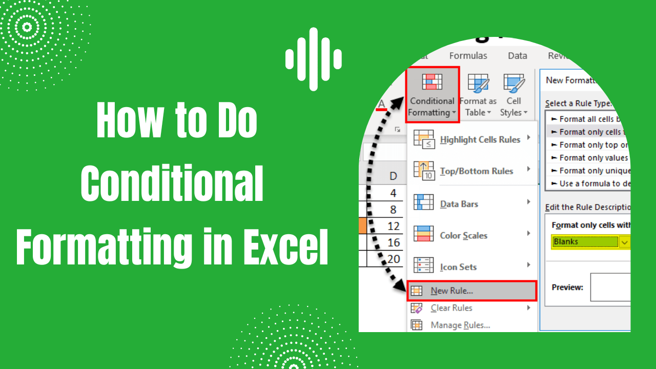 1280×720 conditional formatting excel conditional from earnandexcel.com
  1000×1500 conditional formatting function excel microsoft from www.pinterest.com
  0 x 0 excel conditional formatting based cell video from www.ablebits.com