How To Highlight Top 3 Values In Excel Column
Highlighting the Top 3 Values in an Excel Column
Microsoft Excel is a powerful tool for data analysis and visualization. A common task is to highlight specific values within a dataset to draw attention to important trends or outliers. This guide will walk you through various methods to highlight the top 3 values in a column of data in Excel, from simple conditional formatting to more advanced techniques using formulas and VBA (Visual Basic for Applications).
Method 1: Conditional Formatting – Top/Bottom Rules
The easiest and most straightforward way to highlight the top 3 values is to use Excel’s built-in conditional formatting feature. This method requires no formulas and can be applied directly to your data range.
Steps:
- Select the Data Range: Start by selecting the entire column or the specific range of cells that contain the data you want to analyze. Ensure you’re selecting only the numerical data and not any headers (unless you want them included in the ranking, which is generally not desired).
- Access Conditional Formatting: Go to the “Home” tab on the Excel ribbon. In the “Styles” group, click on the “Conditional Formatting” button. A dropdown menu will appear.
- Choose Top/Bottom Rules: From the dropdown menu, select “Top/Bottom Rules.” Another submenu will appear.
- Select “Top 10 Items…”: From the “Top/Bottom Rules” submenu, select “Top 10 Items…” This option allows you to specify the number of top items you want to highlight.
- Adjust the Number of Items: In the “Top 10 Items” dialog box, change the “10” to “3”. This tells Excel to highlight the top 3 values.
- Choose a Formatting Style: In the same dialog box, you’ll see a dropdown menu labeled “with”. This menu allows you to choose a pre-defined formatting style (e.g., Light Red Fill with Dark Red Text, Yellow Fill with Dark Yellow Text, Green Fill with Dark Green Text) or create a custom format.
- Custom Formatting (Optional): If you want a specific formatting style, select “Custom Format…” from the “with” dropdown menu. This will open the “Format Cells” dialog box, allowing you to customize the font, border, fill, and number formatting of the highlighted cells. For example, you might choose a specific background color or bold font.
- Confirm and Apply: Click “OK” to close the “Top 10 Items” dialog box and apply the conditional formatting to your selected data range.
Advantages:
- Simplicity: This method is extremely easy to use and requires no knowledge of Excel formulas.
- Dynamic: The formatting automatically updates whenever the data in the selected range changes. If a new value becomes one of the top 3, it will be highlighted, and a previously highlighted value will lose its formatting if it falls out of the top 3.
- Predefined Styles: You can quickly apply predefined formatting styles without needing to create custom formats.
Disadvantages:
- Ties: If there are multiple values tied for the 3rd position, only some of them might be highlighted. Excel’s “Top 10 Items” rule doesn’t automatically handle ties in a consistent manner; it may highlight more than 3 cells if ties exist. To reliably handle ties, you’ll need a more complex approach (see Method 3).
- Limited Customization: While you can customize the formatting, the basic rule is limited to highlighting the top N values. More complex criteria require different approaches.
Method 2: Conditional Formatting with RANK.EQ Function
This method utilizes the `RANK.EQ` function to determine the rank of each value within the selected range. By combining `RANK.EQ` with conditional formatting, you can ensure that only the top 3 values (including ties) are highlighted.
Steps:
- Select the Data Range: As before, select the column or range of cells containing the data.
- Access Conditional Formatting: Go to the “Home” tab, click “Conditional Formatting,” and then select “New Rule…”
- Create a New Rule: In the “New Formatting Rule” dialog box, select “Use a formula to determine which cells to format.”
- Enter the Formula: In the formula box, enter the following formula. Assume your data starts in cell A1: `=RANK.EQ(A1, $A$1:$A$100, 0) <= 3` * `A1`: The first cell in your selected data range. Excel will automatically adjust this reference for each cell in the range. * `$A$1:$A$100`: The *absolute* reference to the entire data range. Replace `A100` with the last cell containing data in your column. The `$` signs are crucial to prevent the range from changing as the formula is applied to different cells. * `0`: Specifies that the ranking should be in descending order (largest value gets rank 1). Use `1` for ascending order (smallest value gets rank 1). * `<= 3`: This condition checks if the rank of the current cell is less than or equal to 3. If it is, the cell will be formatted.
- Choose a Formatting Style: Click the “Format…” button to open the “Format Cells” dialog box. Customize the font, border, or fill as desired.
- Confirm and Apply: Click “OK” to close the “Format Cells” dialog box and then click “OK” again to close the “New Formatting Rule” dialog box. The conditional formatting will now be applied to your data range.
Advantages:
- Handles Ties Correctly: This method accurately handles ties. If multiple values are tied for the 3rd position, all of them will be highlighted.
- Formula-Based Flexibility: Using a formula provides greater flexibility for defining the criteria for highlighting. You can easily modify the formula to highlight the top 5, top 10, or any other number of values.
Disadvantages:
- Requires Formula Knowledge: This method requires understanding of the `RANK.EQ` function and absolute vs. relative cell references.
- Slightly More Complex: It’s more involved than the “Top 10 Items” rule, requiring you to create a custom rule and enter a formula.
Method 3: Using the LARGE Function with Conditional Formatting
This method leverages the LARGE function within conditional formatting, providing a more robust and understandable solution for highlighting the top 3 values, especially when dealing with ties.
Steps:
- Select the Data Range: Start by selecting the entire column or the specific range of cells that contains the data you want to highlight.
- Access Conditional Formatting: Go to the “Home” tab, click “Conditional Formatting,” and select “New Rule…”.
- Create a New Rule: In the “New Formatting Rule” dialog box, choose “Use a formula to determine which cells to format.”
- Enter the Formula: Enter the following formula into the formula box. Replace “A1” with the first cell of your data range and “A1:A100” with the entire range.
=A1>=LARGE($A$1:$A$100,3)A1: The first cell in the selected data range. This will be adjusted for each cell in the range.$A$1:$A$100: The absolute reference to the data range. Using$ensures the range doesn’t change as the formula is applied to other cells.LARGE($A$1:$A$100,3): This function returns the 3rd largest value in the range.>=: This checks if the value in cell A1 is greater than or equal to the 3rd largest value. If it is, the cell will be formatted.
- Choose Formatting: Click the “Format…” button to define the desired formatting (fill color, font style, etc.) for the highlighted cells.
- Apply the Rule: Click “OK” in both the “Format Cells” and “New Formatting Rule” dialog boxes. Excel applies the formatting rule to your selected data.
Advantages:
- Accurate Tie Handling: This method reliably highlights all values tied for the top 3, providing a complete and accurate visualization.
- Clarity: The formula is relatively easy to understand, making it maintainable and adaptable.
- Dynamic: Automatically updates the highlights when data changes.
Disadvantages:
- Requires Understanding of LARGE: You need to know how the
LARGEfunction works to use this method effectively. - Slightly More Complex than Top/Bottom Rules: It’s more complex than the “Top 10 Items” method but offers more control.
Method 4: VBA (Visual Basic for Applications)
For more complex scenarios or when you need to automate the highlighting process, you can use VBA. This method requires writing a macro that iterates through the data range and applies formatting based on whether a cell’s value is within the top 3.
Steps:
- Open the VBA Editor: Press Alt + F11 to open the Visual Basic Editor (VBE).
- Insert a Module: In the VBE, go to “Insert” -> “Module”. This will create a new module where you can write your VBA code.
- Write the VBA Code: Copy and paste the following code into the module. Adjust the `DataRange` and `HighlightColor` as needed. “`vba Sub HighlightTop3() Dim DataRange As Range Dim Cell As Range Dim Top3Values As Variant Dim i As Long Dim HighlightColor As Long ‘ Define the data range (adjust as needed) Set DataRange = Range(“A1:A100”) ‘ Replace with your actual data range ‘ Define the highlight color (adjust as needed) HighlightColor = RGB(255, 255, 0) ‘ Yellow ‘ Clear any existing formatting DataRange.Interior.ColorIndex = xlNone ‘ Get the top 3 values Top3Values = Application.WorksheetFunction.Large(DataRange, Array(1, 2, 3)) ‘ Loop through each cell in the data range For Each Cell In DataRange ‘ Check if the cell’s value is in the top 3 For i = LBound(Top3Values) To UBound(Top3Values) If Cell.Value = Top3Values(i) Then Cell.Interior.Color = HighlightColor Exit For ‘ No need to check other top 3 values if already highlighted End If Next i Next Cell End Sub “` * `DataRange`: Change `”A1:A100″` to the actual range of cells containing your data. * `HighlightColor`: Set the desired highlight color using the `RGB` function. You can find RGB color codes online. `RGB(255, 255, 0)` is yellow.
- Run the Macro: In the VBE, go to “Run” -> “Run Sub/UserForm” (or press F5). Alternatively, you can run the macro from the Excel worksheet by pressing Alt + F8, selecting “HighlightTop3” from the list, and clicking “Run”.
Explanation of the VBA Code:
- The code first defines the data range and the highlight color.
- It then clears any existing formatting from the data range to avoid conflicts.
- The `Application.WorksheetFunction.Large` function is used to retrieve the top 3 values from the data range. The `Array(1, 2, 3)` argument tells the function to return the 1st, 2nd, and 3rd largest values.
- The code then iterates through each cell in the data range and checks if its value matches any of the top 3 values. If a match is found, the cell’s background color is changed to the specified highlight color.
Advantages:
- Automation: VBA allows you to automate the highlighting process, which can be useful if you need to perform this task frequently.
- Flexibility: VBA provides the greatest level of flexibility for customizing the highlighting criteria and formatting. You can easily modify the code to handle more complex scenarios or apply different formatting styles.
- Control Over Ties: The VBA code explicitly handles ties by comparing each cell’s value against each of the top 3 values retrieved. This ensures that all cells with a value equal to any of the top 3 values are highlighted.
Disadvantages:
- Requires VBA Knowledge: This method requires knowledge of VBA programming.
- More Complex: Writing and debugging VBA code is more complex than using conditional formatting or formulas.
- Security Considerations: Macros can pose a security risk if they contain malicious code. Be sure to only run macros from trusted sources. You’ll also need to save your Excel file as a macro-enabled workbook (.xlsm).
Conclusion
Highlighting the top 3 values in an Excel column is a common task that can be accomplished using various methods. The best method for you will depend on your level of Excel proficiency, the complexity of your data, and the level of customization you require.
- For simple highlighting and dynamic updates, Conditional Formatting with “Top/Bottom Rules” is the easiest option.
- To accurately handle ties, Conditional Formatting with the RANK.EQ function or LARGE function offers more precision.
- For complex scenarios, automation, and maximum flexibility, VBA is the most powerful solution.
By understanding these different approaches, you can choose the method that best suits your needs and effectively highlight the most important data in your Excel spreadsheets.
 373×366 highlight top values from www.exceldome.com
  624×281 highlight values excel from exceltemplates.net
 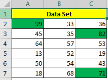 218×162 highlight top values excel from www.exceltip.com
  628×272 highlight highest values column table from datatables.net
  613×377 highlightconditional formatting top values excel from www.extendoffice.com
 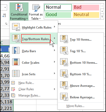 402×427 highlight top bottom values excel list contextures blog from contexturesblog.com