How To Group Time Intervals In Excel Charts
Grouping Time Intervals in Excel Charts
Excel’s charting capabilities are powerful, but working with time-based data can sometimes require manipulation to achieve the desired visualization. When your data contains granular time intervals (seconds, minutes), directly plotting all data points can result in cluttered charts that are difficult to interpret. Grouping these intervals into larger, more meaningful units (hours, days, weeks, months) allows for clearer trends and insights. This document outlines several methods for grouping time intervals in Excel charts, covering different scenarios and techniques.
Understanding the Data
Before grouping, it’s crucial to understand your data. Is the time information stored as a true Excel date/time value, or as text? Excel treats dates and times as numerical values, making calculations and grouping much easier. If your time data is text, you’ll need to convert it to a proper date/time format using functions like DATE, TIME, DATEVALUE, TIMEVALUE, or TEXT. Verify the data’s format using the CELL function with the “format” argument to confirm if Excel recognizes it as a date/time value. Also consider the range and resolution of your time data (e.g., every minute, every hour, daily). This dictates the most appropriate grouping method.
Methods for Grouping Time Intervals
-
Using PivotTables
PivotTables are often the most efficient and flexible way to group time intervals, especially for summarization and aggregation. Here’s how:
- Create a PivotTable: Select your data range (including the time column) and go to Insert > PivotTable. Choose where you want to place the PivotTable (new worksheet or existing location).
- Add Fields: Drag the time field to the “Rows” area and the data you want to analyze (e.g., sales, temperature) to the “Values” area.
- Group the Time Field: Right-click on any date/time in the PivotTable’s row labels and select “Group…”. A dialog box appears allowing you to choose the grouping interval.
- Select Grouping Intervals: Choose from options like Seconds, Minutes, Hours, Days, Months, Quarters, Years. You can select multiple intervals simultaneously (e.g., group by both Months and Days).
- Adjust Start and End Dates: The grouping dialog allows you to specify the starting and ending dates for the grouping. This is useful if you want to start the grouping from a specific point in time.
- Summarize Values: By default, the PivotTable will likely sum the values. You can change the summary function (e.g., average, count, max, min) by clicking the dropdown arrow next to the field name in the “Values” area and selecting “Value Field Settings…”.
- Create a PivotChart: With your PivotTable selected, go to Insert > Charts and choose a chart type (e.g., Line, Column). The chart will automatically reflect the grouped data from the PivotTable.
Advantages: PivotTables offer dynamic grouping. Changing the grouping interval automatically updates both the table and the chart. They also handle aggregation (sum, average, etc.) seamlessly. It provides a ready to use chart.
Disadvantages: PivotTables might be overkill for simple grouping scenarios. They introduce an intermediary table, which might not be desired in all cases.
-
Using Formulas and Helper Columns
When you need more control over the grouping or prefer not to use PivotTables, formulas and helper columns are a good option. This approach involves creating new columns in your data to define the grouped time intervals.
- Create a Helper Column: Insert a new column next to your time column. This column will contain the grouped time values.
- Apply a Formula: Use formulas to round or truncate the time values to the desired interval. Here are some examples:
- Grouping to the Nearest Hour:
=HOUR(A2)(where A2 is the cell containing the time value) will extract the hour component. If you need the date as well, use:=INT(A2) + HOUR(A2)/24. Then format the cell as a date and time. - Grouping to the Nearest Day:
=INT(A2)(where A2 is the cell containing the time value). Format the cell as a date. - Grouping to the Nearest Week (starting Monday):
=A2-WEEKDAY(A2,2)+1. This subtracts the day of the week (1 for Monday, 2 for Tuesday, etc.) from the date, effectively giving you the date of the Monday of that week. Format the cell as a date. - Grouping to the Nearest Month:
=DATE(YEAR(A2),MONTH(A2),1). This creates a date value for the first day of the month containing the original date. Format the cell as a date. - Grouping to Custom Intervals (e.g., every 15 minutes):
=FLOOR(A2, TIME(0,15,0)). This rounds the time down to the nearest multiple of 15 minutes. Change `TIME(0,15,0)` to your desired interval.
- Grouping to the Nearest Hour:
- Create a Summary Table: Create another table summarizing your data based on the grouped time intervals. Use functions like
COUNTIF,SUMIF,AVERAGEIFto aggregate the data from the original data range based on the grouped time in the helper column. For example, if you grouped by hour in column B and want to sum the values in column C for each hour, you could use=SUMIF(B:B, E2, C:C), where E2 contains the hour value you’re summing for. - Create a Chart: Select the data from your summary table (the grouped time intervals and the aggregated values) and insert a chart.
Advantages: Offers precise control over the grouping logic. No dependency on PivotTables. Allows for more complex calculations and transformations within the formulas.
Disadvantages: Requires creating and maintaining formulas, which can be error-prone. Less dynamic than PivotTables; changes to the grouping interval require modifying the formulas. Involves manual creation of a summary table.
-
Using Power Query (Get & Transform Data)
Power Query is a powerful data transformation tool built into Excel. It allows you to import, clean, and transform data from various sources, including Excel tables. Its grouping capabilities are robust and flexible.
- Load Data into Power Query: Select your data range and go to Data > From Table/Range. This opens the Power Query Editor.
- Transform the Data:
- If your date/time column isn’t recognized as a date/time, change its data type by clicking the icon in the column header and selecting “Date/Time” or “Date”.
- Group by Time: Select the date/time column and go to Transform > Date or Transform > Time. Here you’ll find options to extract specific components (Year, Month, Day, Hour, Minute, Second) or perform rounding to specific intervals (e.g., “Hour”, “Beginning of Month”). Choose the option that best suits your grouping needs.
- **Alternatively, using “Group By”:** Go to *Home > Group By*. Choose your grouping time column as the “Basic” field. Give a new name to the resulting column, choose the operation like “Sum” or “Average” and select the data you wish to aggregate.
- Load the Transformed Data: Go to Home > Close & Load > Close & Load To… Choose where you want to load the transformed data (e.g., a new worksheet).
- Create a Chart: Select the grouped data and insert a chart.
Advantages: Powerful data transformation capabilities. Handles various data sources seamlessly. Non-destructive transformations; the original data remains untouched. Allows for complex data cleaning and shaping before grouping. Changes to data update the chart after refreshing the query.
Disadvantages: Steeper learning curve compared to formulas or PivotTables. The initial setup might take longer. It produces another table that needs to be maintained.
Example Scenario: Grouping by Hourly Intervals
Suppose you have a dataset of website traffic recorded every minute, and you want to create a chart showing the hourly traffic trends. Here’s how you could approach it using the methods described above:
- PivotTable: Create a PivotTable with the time field in the Rows area and traffic volume in the Values area. Group the time field by Hours. The resulting PivotTable shows total traffic for each hour.
- Formulas: Add a helper column with the formula
=INT(A2) + HOUR(A2)/24(assuming A2 contains the minute-level time data). Then, create a summary table usingSUMIFto calculate the total traffic for each hour based on the helper column. - Power Query: Load the data into Power Query, change the data type of the time column to Date/Time, and use the “Transform > Time > Hour” option to extract the hour. Group By the “Hour” column with the desired aggregation. Load the transformed data back into Excel.
Tips and Considerations
- Data Consistency: Ensure that your time data is consistent. Inconsistencies (e.g., missing data points, irregular intervals) can affect the accuracy of the grouping and subsequent analysis.
- Chart Types: Choose appropriate chart types for time series data. Line charts are generally suitable for showing trends over time. Column charts are useful for comparing values at different points in time. Scatter plots can be used to visualize the relationship between time and other variables.
- Chart Axis Formatting: Format the chart’s horizontal axis to display time values in a readable format. Right-click on the axis and select “Format Axis…”. Adjust the number format and axis options as needed.
- Blank cells: Grouping will treat blank cells in the source data as zero or ignore them, depending on the aggregation method used. Handle blank cells appropriately based on the desired analysis.
- Large Datasets: For very large datasets, Power Query is generally the most efficient method for grouping and transforming time intervals.
- Dynamic Updates: When your source data changes frequently, consider using PivotTables or Power Query, as they can be easily refreshed to reflect the latest data.
Conclusion
Grouping time intervals in Excel charts is essential for visualizing and analyzing time-based data effectively. By understanding the different methods available (PivotTables, formulas, Power Query) and their respective advantages and disadvantages, you can choose the most appropriate approach for your specific needs. Remember to consider data consistency, chart type selection, and axis formatting to create clear and informative visualizations that reveal valuable insights.
 287×302 group time minutes hours intervals excel from www.extendoffice.com
  560×428 ways group times excel excel campus from www.excelcampus.com
 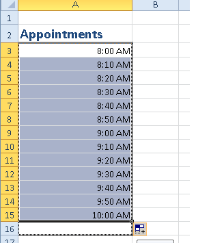 309×355 easily create sequence regularly spaced time intervals excel from howtoexcelatexcel.com