How To Find And Highlight Blank Cells In Excel
Finding and Highlighting Blank Cells in Excel
Blank cells in Excel spreadsheets can be more than just visually empty spaces; they can represent missing data, errors in calculations, or inconsistencies in your dataset. Identifying and addressing these blank cells is crucial for accurate analysis, reliable reporting, and effective data management. This guide provides a comprehensive overview of various methods to find and highlight blank cells in Excel, catering to different scenarios and user skill levels.
Why Find and Highlight Blank Cells?
Before diving into the techniques, understanding the importance of locating blank cells is essential:
- Data Integrity: Blank cells can skew calculations, leading to inaccurate results. For example, averaging a column with blank cells can produce a different result than averaging the same column after replacing blanks with zeros.
- Data Consistency: Identifying blank cells allows you to enforce data consistency. You can ensure that all entries in a specific column are complete, adhering to a defined data structure.
- Error Detection: Blank cells might indicate errors in data entry or data migration. Finding them can help you trace the source of the error and correct it.
- Reporting Accuracy: Blank cells in reports can be confusing or misleading. Highlighting them helps you quickly identify areas requiring attention and ensures clarity in your presentations.
- Data Cleaning: Blank cells are often the first step in data cleaning. Once identified, you can decide how to handle them – filling them with appropriate values, deleting the rows, or leaving them as is with a specific designation.
Methods to Find Blank Cells
Excel offers several methods to locate blank cells, ranging from simple manual inspection to advanced filtering and formula-based approaches.
1. Manual Inspection
For smaller datasets, a simple visual scan can be sufficient to identify blank cells. However, this method is impractical and error-prone for large spreadsheets.
When to use: Small datasets, quick checks, when you are only concerned about specific areas of the spreadsheet.
Limitations: Time-consuming, prone to human error, unsuitable for large datasets.
2. Go To Special
The “Go To Special” feature is a powerful and efficient way to select all blank cells within a selected range.
Steps:
- Select the range of cells you want to examine. To check the entire sheet, click the small square at the intersection of the row and column headers.
- Go to the “Home” tab.
- In the “Editing” group, click “Find & Select”.
- Choose “Go To Special…”.
- In the “Go To Special” dialog box, select “Blanks”.
- Click “OK”.
Excel will select all the blank cells within the chosen range. Now you can apply formatting (e.g., highlight with a color) or perform other actions on the selected cells.
When to use: Medium to large datasets, when you need to select and format blank cells quickly.
Advantages: Fast, accurate, allows for quick selection of all blank cells.
Limitations: Requires selecting the range first, doesn’t dynamically update as data changes (you’ll need to repeat the process).
3. Filter by Blanks
The filtering feature allows you to isolate rows containing blank cells in a specific column.
Steps:
- Select the column you want to filter.
- Go to the “Data” tab.
- Click “Filter”. This will add dropdown arrows to the column headers.
- Click the dropdown arrow in the column you selected.
- In the filter menu, uncheck “Select All”.
- Scroll down and check the “(Blanks)” option.
- Click “OK”.
Excel will display only the rows where the selected column contains blank cells. You can then highlight these rows or perform other operations.
When to use: When you need to identify entire rows containing blank cells in a specific column, especially useful for data cleaning and validation.
Advantages: Easy to use, allows for isolating rows with blank cells in a particular column.
Limitations: Only filters one column at a time, hides other rows, doesn’t directly highlight blank cells.
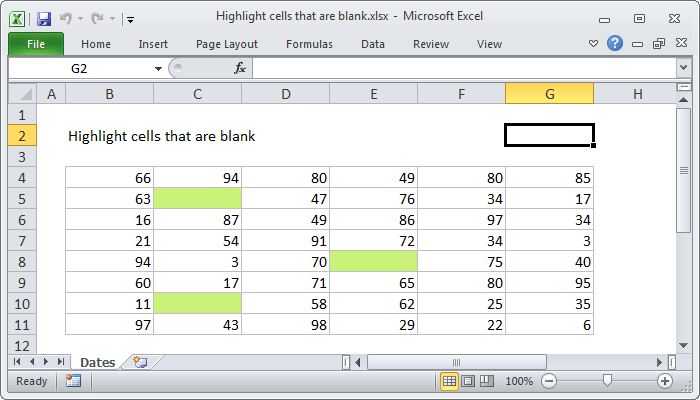
4. Conditional Formatting with Formulas
Conditional formatting lets you dynamically highlight blank cells based on a formula. This is particularly useful when your data is frequently updated.
Steps:
- Select the range of cells you want to format.
- Go to the “Home” tab.
- In the “Styles” group, click “Conditional Formatting”.
- Choose “New Rule…”.
- In the “New Formatting Rule” dialog box, select “Use a formula to determine which cells to format”.
- In the “Format values where this formula is true” box, enter the formula `=ISBLANK(A1)` (replace `A1` with the address of the top-left cell in your selected range). Make sure the cell reference is relative (no dollar signs).
- Click the “Format…” button.
- Choose the desired fill color or other formatting options on the “Fill” tab.
- Click “OK” to close the “Format Cells” dialog box.
- Click “OK” to close the “New Formatting Rule” dialog box.
This will highlight all blank cells within the selected range. The highlighting will automatically update as cells are populated or cleared.
When to use: When you need dynamic highlighting that updates automatically as data changes, complex scenarios involving multiple conditions.
Advantages: Dynamic highlighting, formula-based, allows for complex criteria.
Limitations: Requires understanding of Excel formulas, can slow down performance on very large datasets if the formula is complex.
5. Using the COUNTBLANK Function
The `COUNTBLANK` function counts the number of empty cells in a range. While it doesn’t directly highlight cells, it’s useful for assessing the extent of blank cells in your data.
Syntax: `=COUNTBLANK(range)`
For example, `=COUNTBLANK(A1:A100)` will count the number of blank cells in the range A1 to A100.
You can combine `COUNTBLANK` with conditional formatting to highlight cells based on the *presence* of blanks within a range, but it won’t highlight *individual* blank cells directly. Instead, you might highlight a cell if `COUNTBLANK(A1:A100)>0`, indicating that there are blank cells in that range.
When to use: When you need to quantify the number of blank cells, to use the count in other calculations or formulas, or to trigger conditional formatting based on the presence of blanks.
Advantages: Simple, provides a numerical count of blank cells.
Limitations: Doesn’t directly highlight blank cells, only counts them.
6. Combining Formulas with Conditional Formatting (Advanced)
You can create more sophisticated conditional formatting rules by combining formulas with conditional formatting. For example, you might want to highlight only blank cells in specific columns or rows based on values in other cells.
Example: Highlight blank cells in column B only if the corresponding cell in column A contains the word “Error”.
Formula: `=AND(ISBLANK(B1),A1=”Error”)`
Apply this formula using the conditional formatting steps outlined above, replacing `A1` and `B1` with the appropriate starting cells for your range.
When to use: Complex scenarios requiring conditional highlighting based on multiple criteria.
Advantages: Highly flexible, allows for customized highlighting based on specific conditions.
Limitations: Requires advanced Excel knowledge, can be complex to implement.
Choosing the Right Method
The best method for finding and highlighting blank cells depends on your specific needs and the size and complexity of your data:
- Small Datasets: Manual inspection or “Go To Special” may suffice.
- Medium to Large Datasets: “Go To Special”, filtering, or conditional formatting are more efficient.
- Dynamic Highlighting: Conditional formatting with formulas is the preferred choice.
- Specific Column Focus: Filtering is ideal for isolating rows with blank cells in a particular column.
- Quantifying Blank Cells: Use the `COUNTBLANK` function.
- Complex Criteria: Combine formulas with conditional formatting.
Beyond Highlighting: Handling Blank Cells
Highlighting blank cells is just the first step. You’ll also need to decide how to handle them:
- Fill with Zero: If the blank cell represents a zero value, replace it with 0.
- Fill with a Default Value: If the blank cell represents a missing value with a known default, replace it with that value.
- Fill with Interpolated Values: If the data follows a trend, you can use interpolation techniques to estimate the missing value.
- Leave as Blank: In some cases, it may be appropriate to leave the blank cell as is, especially if it represents a truly unknown or inapplicable value.
- Delete the Row or Column: If the blank cell represents a significant missing piece of information that cannot be recovered, you may need to delete the entire row or column. Be cautious with this approach, as it can lead to data loss.
- Replace with a Placeholder: Replacing blank cells with a specific placeholder (e.g., “N/A”, “Missing”, “Unknown”) can be useful for indicating that the value is intentionally missing.
Remember to carefully consider the implications of each approach before making changes to your data. Documenting your data cleaning decisions is also crucial for maintaining data integrity and reproducibility.
Conclusion
Finding and highlighting blank cells in Excel is a fundamental skill for data analysis and management. By mastering the techniques outlined in this guide, you can effectively identify and address blank cells in your spreadsheets, ensuring the accuracy and reliability of your data.
 700×400 excel formula highlight blank cells exceljet from exceljet.net
  415×422 highlight blank cells excel seconds from trumpexcel.com
 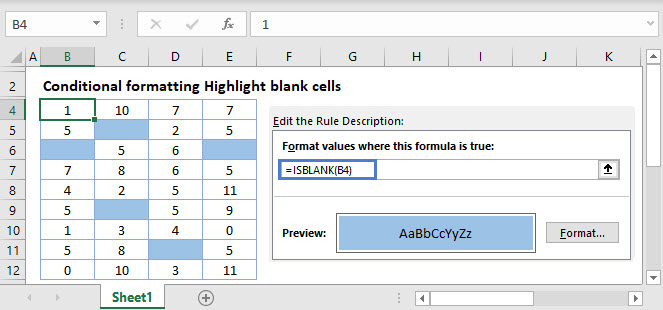 663×310 highlight blank cells conditional formatting automate excel from www.automateexcel.com