How To Create Dynamic Dropdown List With Search In Excel
“`html
Creating Dynamic Dropdown Lists with Search Functionality in Excel
Excel’s data validation feature is incredibly useful for creating dropdown lists, ensuring data consistency, and streamlining data entry. However, a standard dropdown becomes cumbersome with large datasets. A dynamic dropdown list with a search function offers a more efficient and user-friendly solution, allowing users to quickly find and select the desired option from a vast list.
Why Use a Dynamic Searchable Dropdown?
- Improved User Experience: Users can quickly locate items by typing, eliminating the need to scroll through long lists.
- Enhanced Data Accuracy: Restricts data entry to predefined values, minimizing errors and inconsistencies.
- Greater Efficiency: Speeds up data entry, saving time and effort.
- Scalability: Works seamlessly with both small and large datasets.
Steps to Create a Dynamic Searchable Dropdown in Excel
This guide outlines a method using named ranges and a helper column to achieve this functionality. We’ll be using Excel’s built-in functions and avoiding VBA (Visual Basic for Applications) for simplicity.
1. Prepare Your Data
First, organize your data into a single column. This column will serve as the source for your dropdown list. Ensure there are no blank cells within the data range, as this can disrupt the functionality.
Example: Imagine you have a list of customer names in column A, starting from A2. A1 could contain the header “Customer Name”.
2. Create a Named Range for Your Data
Defining a named range makes your formula more readable and easier to maintain.
- Select the entire range of your data, including the header. In our example, select from A1 to the last row containing a customer name.
- Go to the “Formulas” tab on the Excel ribbon.
- Click “Define Name” in the “Defined Names” group.
- In the “New Name” dialog box:
- Enter a name for your range in the “Name” field. A descriptive name like “CustomerList” is recommended.
- Ensure the “Refers to” field correctly points to your selected data range (e.g.,
=$A$1:$A$100). - Click “OK”.
3. Create a Search Box
Designate a cell where the user will type their search query. This cell will drive the filtering of the dropdown list. Let’s say you choose cell C2 for the search box and label C1 as “Search”.
4. Create a Helper Column with a Filtering Formula
This is the core of the dynamic functionality. We’ll use a formula in a helper column to identify items in your data that match the search query. It’s common practice to place this helper column away from your main data.
- Choose a column for your helper column (e.g., column B). Start the formula in the first row *below* your header row in the original data column (in our case, B2).
- Enter the following formula in cell B2:
=IF(ISERROR(SEARCH($C$2,A2)),"",A2)$C$2: This is the absolute reference to the search box cell. The$symbols ensure that this reference doesn’t change when you copy the formula down the column.A2: This is the relative reference to the corresponding cell in your data column (the column with customer names).SEARCH($C$2,A2): This function searches for the text entered in the search box ($C$2) within the current cell in the data column (A2). It returns the starting position of the search text if found, and an error if not found. This function is not case-sensitive.ISERROR(SEARCH($C$2,A2)): This checks if theSEARCHfunction returned an error. If it did (meaning the search term was not found), this will returnTRUE.IF(ISERROR(SEARCH($C$2,A2)),"",A2): This is the conditional statement. If the search term is *not* found (ISERRORreturnsTRUE), the cell in the helper column will be left blank (""). If the search term *is* found (ISERRORreturnsFALSE), the cell will display the value from the corresponding cell in the data column (A2).
- Copy the formula down the entire length of your data range. You can do this by clicking the small square at the bottom-right corner of cell B2 and dragging it down, or by double-clicking the square if the adjacent column (column A in this case) has data in every row.
5. Create a Named Range for the Filtered List
Now we need to create a dynamic named range that only includes the values from the helper column that are not blank (i.e., the values that match the search query). We’ll use the OFFSET and COUNTA functions for this.
- Go to the “Formulas” tab on the Excel ribbon.
- Click “Define Name” in the “Defined Names” group.
- In the “New Name” dialog box:
- Enter a name for this range, such as “FilteredCustomerList”.
- In the “Refers to” field, enter the following formula:
=OFFSET($B$2,0,0,COUNTA($B:$B)-1,1)OFFSET($B$2,0,0,COUNTA($B:$B)-1,1): This function creates a dynamic range.$B$2: This is the starting point of the range (the first cell in your helper column *below* the header).0,0: These represent the number of rows and columns to offset from the starting cell. In this case, we don’t want to offset at all, so both are 0.COUNTA($B:$B)-1: This calculates the height of the range (the number of rows).COUNTA($B:$B)counts all non-blank cells in column B, including the header row (if any). Subtracting 1 removes the header row, giving you the correct number of rows for your filtered data.1: This specifies the width of the range (number of columns). Since our filtered list is in a single column, the width is 1.
- Click “OK”.
6. Create the Data Validation Dropdown
Finally, create the data validation dropdown using the dynamic named range we just defined.
- Select the cell where you want the dropdown list to appear. Let’s say you choose cell D2 and label D1 as “Select Customer”.
- Go to the “Data” tab on the Excel ribbon.
- Click “Data Validation” in the “Data Tools” group.
- In the “Data Validation” dialog box:
- On the “Settings” tab:
- In the “Allow” dropdown, select “List”.
- In the “Source” field, enter
=FilteredCustomerList(the name of your filtered data range). - (Optional) Check the “Ignore blank” checkbox to prevent blank options from appearing in the dropdown.
- (Optional) Check the “In-cell dropdown” checkbox to display the dropdown arrow.
- (Optional) On the “Input Message” tab, you can add a helpful message that appears when the cell is selected.
- (Optional) On the “Error Alert” tab, you can customize the error message that appears if a user enters a value that is not in the list.
- Click “OK”.
- On the “Settings” tab:
7. Test Your Dynamic Dropdown
Now you can test your dynamic dropdown list. Type a search term into the search box (cell C2). The dropdown list in cell D2 should now only show items that match your search query. Clear the search box to see the entire list again.
Tips and Considerations
- Case Sensitivity: The
SEARCHfunction is not case-sensitive. If you need a case-sensitive search, use theFINDfunction instead. - Large Datasets: For very large datasets, consider using more advanced techniques like VBA to optimize performance.
- Error Handling: Implement error handling to gracefully handle situations where the search term is not found or the data is invalid.
- Data Updates: If your data changes frequently, ensure the named ranges and formulas are updated accordingly. Using dynamic named ranges (as demonstrated above with the `OFFSET` and `COUNTA` functions) helps automate this.
- Formatting: Format your cells and ranges for better readability and aesthetics.
By following these steps, you can create a dynamic dropdown list with search functionality in Excel, making data entry more efficient and user-friendly.
“`
 1280×720 create searchable dropdown list excel excel microsoft excel from www.pinterest.com
  1334×993 create dynamic drop list excel excel unlocked from excelunlocked.com
  920×746 create dynamic drop list excel from www.skyxcel.com
 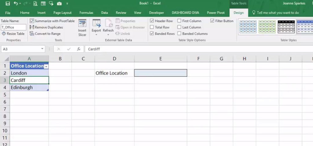 1024×478 create dynamic drop list excel expedio data design from expediodata.design
 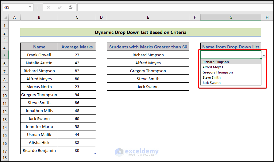 893×529 dynamic list excel complete guideline exceldemy from www.exceldemy.com
  422×323 dropdown list excel puresourcecode from www.puresourcecode.com
 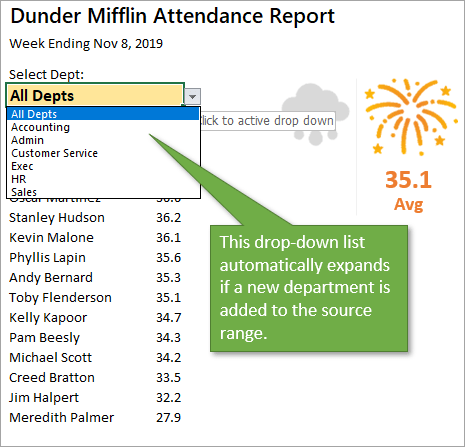 465×447 create dynamic drop list automatically expands from www.excelcampus.com
  1000×750 dropdowns excel google sheets searchable dynamic upwork from www.upwork.com
  1280×720 create dynamic drop list excel vba printable from tupuy.com
 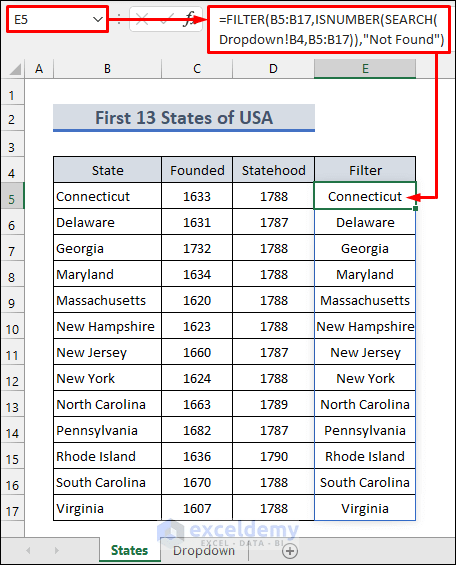 456×565 create searchable drop list excel methods exceldemy from www.exceldemy.com
  473×841 searchable drop list excel dynamic search data validation list from www.artofit.org
 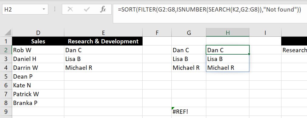 1012×389 set searchable dropdown list fix excel errors from fixallexcelerrors.com
  480×360 create dynamic searchable drop list excel artofit from www.artofit.org
  510×295 create searchable drop list excel methods from www.excel-end.com
  597×518 ultimate guide searchable drop list excel from www.extendoffice.com
  587×525 create searchable drop list excel from www.extendoffice.com
  1221×841 part create searchable drop list microsoft excel from www.exceldoctor.be
  430×480 create excel drop list search suggestions from trumpexcel.com
  630×388 create searchable drop list excel from www.bizinfograph.com
  1280×720 easy drop list excel from fity.club