How To Create An Index Match Formula In Excel
Creating Index Match Formulas in Excel: A Comprehensive Guide
The INDEX MATCH formula is a powerful and flexible alternative to VLOOKUP and HLOOKUP in Excel. It overcomes the limitations of VLOOKUP, offering greater accuracy and adaptability when searching for data within your spreadsheets. This guide will walk you through the intricacies of creating and using INDEX MATCH formulas, covering everything from the basic syntax to more advanced applications.
Understanding the Limitations of VLOOKUP
Before diving into INDEX MATCH, it’s important to understand why it’s often preferred over VLOOKUP. VLOOKUP (Vertical Lookup) has two main limitations:
- Column Restriction: VLOOKUP can only search for a value in the leftmost column of the specified range. This means the column containing the value you want to return must be to the right of the lookup column.
- Insertion/Deletion Issues: When you insert or delete columns within the VLOOKUP range, the column index number (the third argument in the formula) might change, causing the formula to return incorrect results.
INDEX MATCH addresses these limitations, offering a more robust and adaptable solution.
The INDEX MATCH Formula: Breaking It Down
The INDEX MATCH formula combines two separate Excel functions: INDEX and MATCH. Let’s examine each individually before combining them.
INDEX Function
The INDEX function returns the value of a cell within a specified range based on its row and column numbers. The basic syntax is:
=INDEX(array, row_num, [column_num])
- array: The range of cells from which you want to return a value.
- row_num: The row number within the array from which to return a value.
- [column_num]: (Optional) The column number within the array from which to return a value. If omitted, the INDEX function assumes you are working with a single-column array.
Example: =INDEX(A1:C10, 5, 2) will return the value in the cell at the intersection of the 5th row and 2nd column within the range A1:C10. This corresponds to cell B5.
MATCH Function
The MATCH function returns the relative position of a specified value within a range of cells. The basic syntax is:
=MATCH(lookup_value, lookup_array, [match_type])
- lookup_value: The value you are trying to find.
- lookup_array: The range of cells where you want to search for the lookup_value.
- [match_type]: (Optional) Specifies how MATCH should find the lookup_value. The options are:
- 0: (Exact Match) Finds the first value that is exactly equal to the lookup_value. This is the most common and recommended option for most lookup scenarios.
- 1: (Less Than) Finds the largest value that is less than or equal to the lookup_value. The lookup_array must be sorted in ascending order for this to work correctly.
- -1: (Greater Than) Finds the smallest value that is greater than or equal to the lookup_value. The lookup_array must be sorted in descending order for this to work correctly.
If omitted, match_type defaults to 1.
Example: =MATCH("Apple", A1:A10, 0) will search for the value “Apple” within the range A1:A10 and return the row number where “Apple” is found. If “Apple” is in cell A3, the formula will return 3.
Combining INDEX and MATCH
The power of INDEX MATCH lies in using the MATCH function to dynamically determine the row number for the INDEX function. Instead of hardcoding the row number, MATCH finds the row containing the lookup value.
The general syntax for a basic INDEX MATCH formula is:
=INDEX(return_array, MATCH(lookup_value, lookup_array, 0))
- return_array: The range of cells containing the values you want to return.
- lookup_value: The value you want to search for.
- lookup_array: The range of cells where you want to search for the lookup_value.
- 0: Specifies an exact match for the MATCH function.
Example: Imagine you have a table with employee names in column A (A2:A10) and their corresponding salaries in column B (B2:B10). You want to find the salary of the employee named “Jane Doe”.
The INDEX MATCH formula would be:
=INDEX(B2:B10, MATCH("Jane Doe", A2:A10, 0))
Here’s how it works:
MATCH("Jane Doe", A2:A10, 0)searches for “Jane Doe” in the range A2:A10 and returns the row number where “Jane Doe” is found (e.g., if “Jane Doe” is in A5, it returns 4).INDEX(B2:B10, 4)then uses that row number (4) to return the value in the 4th row of the range B2:B10, which is Jane Doe’s salary.
Advantages of INDEX MATCH Over VLOOKUP
- Flexible Lookup Direction: INDEX MATCH can search for a value in any column within your data range. The return column doesn’t have to be to the right of the lookup column.
- Column Insertion/Deletion Resilience: If you insert or delete columns, the INDEX MATCH formula will still work correctly because it relies on range names or absolute references, not fixed column index numbers.
- Improved Performance: In some cases, INDEX MATCH can be slightly faster than VLOOKUP, especially with large datasets. This is because VLOOKUP checks every row in the lookup array, whereas INDEX MATCH directly accesses the target row once the match is found.
Advanced INDEX MATCH Applications
Beyond the basic example, INDEX MATCH can be used in more sophisticated ways.
Two-Way Lookup (INDEX MATCH MATCH)
This allows you to look up values based on both row and column criteria, similar to using both VLOOKUP and HLOOKUP simultaneously. Imagine you have a table showing sales figures for different products across different months. You want to find the sales figure for a specific product in a specific month.
The formula would look like this:
=INDEX(data_range, MATCH(row_lookup_value, row_lookup_range, 0), MATCH(column_lookup_value, column_lookup_range, 0))
- data_range: The entire range containing the sales figures.
- row_lookup_value: The product name you want to find.
- row_lookup_range: The range containing the product names (e.g., A2:A10).
- column_lookup_value: The month you want to find.
- column_lookup_range: The range containing the month names (e.g., B1:M1).
Example: If your data range is B2:M10, product names are in A2:A10, month names are in B1:M1, you want to find the sales of “Product A” in “March”, the formula would be:
=INDEX(B2:M10, MATCH("Product A", A2:A10, 0), MATCH("March", B1:M1, 0))
Using Named Ranges
Using named ranges can make your INDEX MATCH formulas easier to read and maintain. To create a named range, select the range of cells and then type a name in the Name Box (to the left of the formula bar) and press Enter. Then you can use the name in your formula.
For example, if you named the range B2:B10 “Salaries” and A2:A10 “EmployeeNames”, the previous example would become:
=INDEX(Salaries, MATCH("Jane Doe", EmployeeNames, 0))
This is much more readable and less prone to errors.
Handling Errors (IFERROR)
If the lookup value is not found in the lookup array, the MATCH function will return an #N/A error. To handle this, you can wrap the INDEX MATCH formula within an IFERROR function.
The syntax is:
=IFERROR(INDEX(return_array, MATCH(lookup_value, lookup_array, 0)), "Value Not Found")
This will display “Value Not Found” (or any message you choose) if the lookup value isn’t found.
Tips and Best Practices
- Always use an exact match (0) in the MATCH function unless you specifically need an approximate match.
- Use absolute references ($) to lock ranges if you are copying the formula to other cells. For example,
=INDEX($B$2:$B$10, MATCH("Jane Doe", $A$2:$A$10, 0)) - Consider using named ranges for better readability and maintainability.
- Use the IFERROR function to handle potential errors gracefully.
- Double-check your ranges to ensure they are accurate.
Conclusion
The INDEX MATCH formula is an invaluable tool for Excel users seeking a more flexible and robust alternative to VLOOKUP. By understanding the individual functions and how they work together, you can leverage this powerful technique to efficiently and accurately retrieve data from your spreadsheets. Practice with different scenarios and explore the advanced applications to master this essential Excel skill.
 1500×1000 index match formula excel excel hindi from www.excelsuperstar.org
  1366×768 advanced index match formula excel excel hindi from www.excelsuperstar.org
 :max_bytes(150000):strip_icc()/index-match-excel-examples-1b2fc8cd04904f678b0e224f644372be.png) 1302×868 index match function excel xls complete guide from mathformula6.netlify.app
1302×868 index match function excel xls complete guide from mathformula6.netlify.app  700×400 index match function excel complete guide from mathformula5.netlify.app
  1330×749 learn basics index match formula excel part from www.excelsuperstar.org
  361×297 index match match step step excel tutorial from corporatefinanceinstitute.com
  700×400 excel formula index match multiple criteria exceljet from exceljet.net
  623×340 index match excel easy formulas from www.bharatagritech.com
 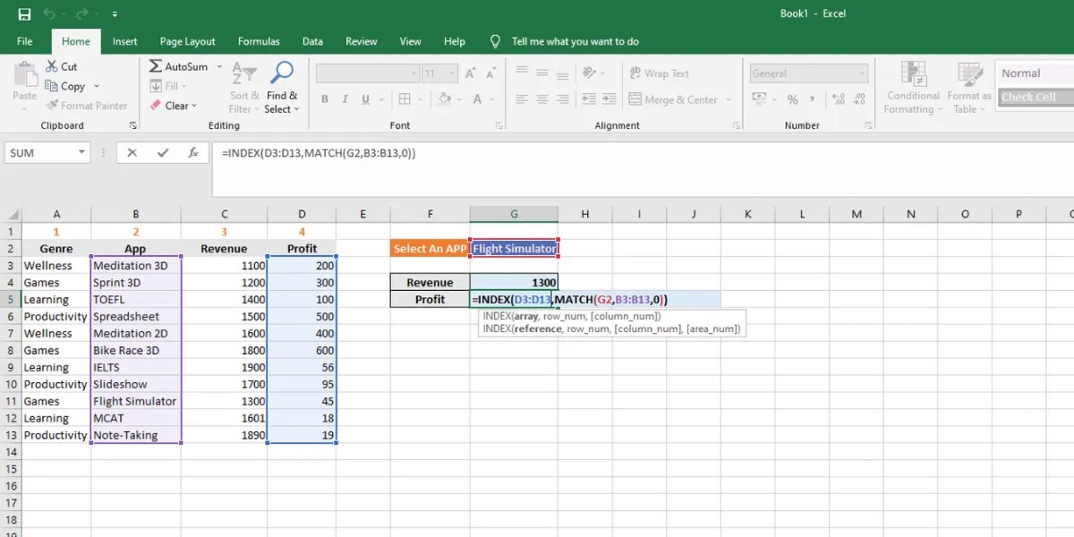 1200×600 index match excel advanced lookups from www.makeuseof.com
 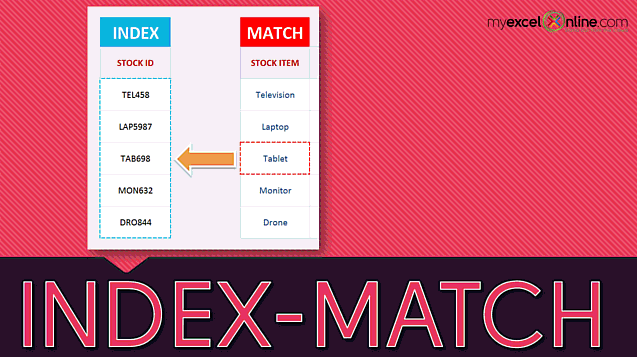 637×357 index match formula myexcelonline from www.myexcelonline.com
  767×452 examples index match formula excel approaches from www.exceldemy.com
 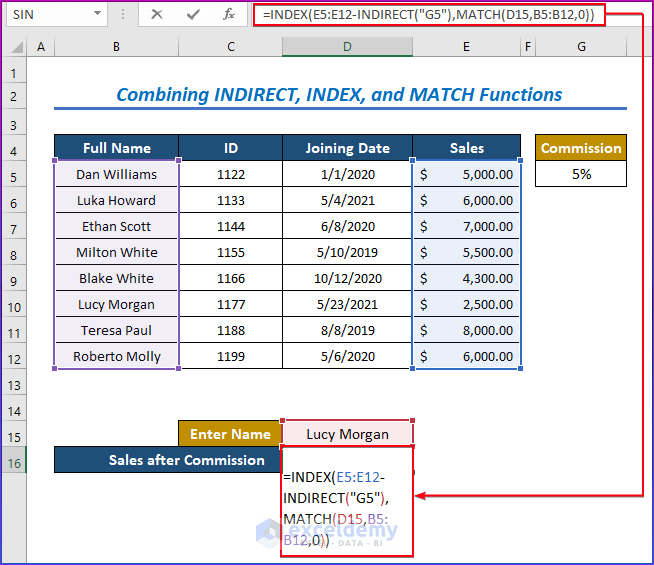 654×565 indirect index match functions excel from www.exceldemy.com
  736×414 index match formula explained excel excel from www.pinterest.com
  800×600 index match excel customguide from www.customguide.com
  768×1054 excel practice exercises index match formula from www.exceldemy.com
 /index-match-combined-f335f7c14de94f27bc0e5c37af3971e0.png) 1089×726 index match function excel from www.lifewire.com
1089×726 index match function excel from www.lifewire.com  1200×630 excel index match criteria media rpgsite from media.rpgsite.net
  679×519 excel functions index match from excel-pratique.com
  481×317 excel index match multiple criteria formula examples from www.ablebits.com
  300×252 index match excel formula guide from excelchamps.com
 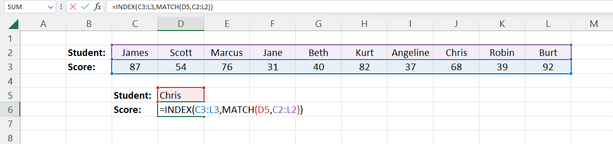 1202×283 index match excel quick guide from fundsnetservices.com
  700×400 index match advanced excel formula exceljet from exceljet.net
 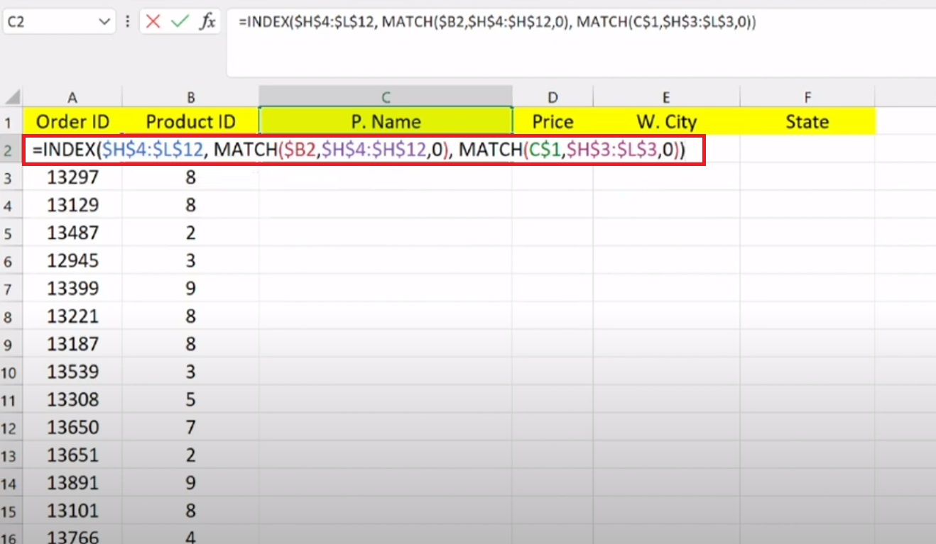 1318×767 index match function excel powerful flexible from www.exceltutorial.net
  751×271 index match function excel index match function excel from www.educba.com
  700×400 index match multiple columns excel formula exceljet from exceljet.net