How To Create A Checklist With Strikethrough In Excel
“`html
Creating a Checklist with Strikethrough in Excel
Excel’s versatility extends far beyond number crunching; it can also be a powerful tool for managing tasks and creating interactive checklists. A popular technique involves using checkboxes to mark items as complete, automatically applying a strikethrough effect to visually indicate their finished status. This tutorial will guide you through the process of building such a checklist, providing a clear and organized way to track progress.
Setting Up the Foundation: The Checklist Column
Begin by creating a new Excel worksheet or using an existing one. In the first column (e.g., column A), list the tasks or items that need to be included in your checklist. For example:
- Grocery Shopping
- Pay Bills
- Write Report
- Schedule Meeting
- Clean House
Adjust the column width to accommodate the lengthiest task description. This column will display the task list that users interact with.
Inserting Checkboxes: The Developer Tab
The next step involves adding checkboxes adjacent to each task. To do this, you’ll need to access the Developer tab. By default, this tab isn’t visible, so you’ll need to enable it.
- Access Excel Options: Click on the “File” tab in the Excel ribbon, then select “Options” from the menu.
- Customize the Ribbon: In the Excel Options dialog box, choose “Customize Ribbon” from the left-hand menu.
- Enable the Developer Tab: On the right side of the dialog box, under “Customize the Ribbon,” locate “Developer” in the list of main tabs. Check the box next to “Developer” and click “OK.”
The Developer tab should now be visible in your Excel ribbon.
Adding the Checkboxes
With the Developer tab enabled, you can now insert checkboxes next to each task in your list.
- Select the Developer Tab: Click on the newly enabled “Developer” tab in the Excel ribbon.
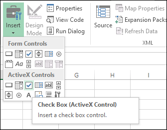
- Insert Control: Within the “Controls” group, click on “Insert.” A dropdown menu will appear.
- Choose Check Box (Form Control): Under “Form Controls,” select the “Check Box (Form Control)” option (it looks like a square with a check mark).
- Draw the Checkbox: Click and drag your mouse in the cell next to the first task (e.g., cell B2) to draw the checkbox. Adjust the size as needed.
- Edit the Checkbox Text: Right-click on the checkbox and select “Edit Text.” Delete the default text (usually “Check Box 1”) so that only the checkbox remains.
- Link the Checkbox to a Cell: This is crucial for the strikethrough functionality. Right-click on the checkbox again and select “Format Control.” In the “Control” tab, under “Cell link,” enter the cell in the same row in a different column (e.g., cell C2). This cell will now display TRUE when the checkbox is checked and FALSE when it’s unchecked. Click “OK.”
- Repeat for Each Task: Repeat steps 4-7 for each task in your checklist, ensuring that each checkbox is linked to a different cell in the same row (e.g., B3 linked to C3, B4 linked to C4, and so on). You can copy and paste the first checkbox to the other rows to save time, but remember to adjust the cell link for each checkbox individually.
You should now have a column of checkboxes next to your task list, and a corresponding column with TRUE/FALSE values reflecting the checkbox states.
Applying the Strikethrough: Conditional Formatting
The final step is to apply conditional formatting that automatically applies a strikethrough to a task when its corresponding checkbox is checked (TRUE). This is where the magic happens.
- Select the Task List: Highlight the entire column containing your task list (e.g., column A).
- Access Conditional Formatting: Click on the “Home” tab in the Excel ribbon. In the “Styles” group, click on “Conditional Formatting.” A dropdown menu will appear.
- Create a New Rule: Select “New Rule…” from the dropdown menu. This opens the New Formatting Rule dialog box.
- Use a Formula: In the “Select a Rule Type” section, choose “Use a formula to determine which cells to format.”
- Enter the Formula: In the “Format values where this formula is true” box, enter the following formula:
=$C2Explanation:
- The
=sign indicates the start of a formula. $C2refers to the cell linked to the checkbox in the first row of your task list. The dollar sign before the “C” makes the column reference absolute (meaning it won’t change when the rule is applied to other rows). The “2” is the row number, and it *must* correspond to the first row in your selected task list.
- The
- Format the Cell: Click on the “Format…” button. This opens the Format Cells dialog box.
- Apply Strikethrough: In the Format Cells dialog box, go to the “Font” tab. Under “Effects,” check the box next to “Strikethrough.”
- Choose a Color (Optional): You can also choose a different font color to further visually distinguish completed tasks.
- Confirm the Formatting: Click “OK” to close the Format Cells dialog box, and then click “OK” again to close the New Formatting Rule dialog box.
Now, when you check a box, the corresponding task in column A should automatically have a strikethrough applied. When you uncheck the box, the strikethrough should disappear.
Customization and Troubleshooting
- Adjusting the Formula: If your task list doesn’t start in row 2, you’ll need to adjust the row number in the formula (e.g., if your tasks start in row 5, the formula would be
=$C5). - Changing the Cell Link Column: If you’re using a different column for the TRUE/FALSE values (the “Cell link” in the checkbox format), change the column letter in the formula accordingly.
- Formatting Consistency: Ensure that the entire task list column is selected when applying conditional formatting to maintain consistency.
- Troubleshooting: If the strikethrough isn’t working, double-check:
- The Developer tab is enabled.
- Checkboxes are correctly inserted.
- Each checkbox is linked to a cell.
- The conditional formatting rule is correctly applied to the task list column.
- The formula in the conditional formatting rule is correct, especially the cell reference.
Beyond the Basics
This checklist functionality can be enhanced further with more advanced Excel features:
- Sorting: Sort the task list by completion status (checked/unchecked) to easily prioritize incomplete tasks. You can use the “Sort” feature on the “Data” tab, sorting by the column containing the TRUE/FALSE values.
- Filtering: Filter the task list to show only incomplete or completed tasks. Use the “Filter” feature on the “Data” tab and filter the column containing the TRUE/FALSE values.
- Progress Tracking: Add a formula to count the number of completed tasks (TRUE values) and calculate the percentage of completion. For example, you can use the `COUNTIF` function: `=COUNTIF(C2:C10,TRUE)` (assuming your TRUE/FALSE values are in the range C2:C10). Then, divide this count by the total number of tasks to get the percentage.
- Visual Cues: Use other conditional formatting rules to highlight urgent tasks or tasks nearing their deadline. For example, use color scales or icon sets based on dates or priority levels in separate columns.
By following these steps, you can create a dynamic and user-friendly checklist in Excel that effectively tracks progress and promotes efficient task management. The combination of checkboxes and conditional formatting provides a clear visual representation of completed tasks, improving organization and productivity.
“`
 335×262 unique ways apply strikethrough excel shortcut command from excelchamps.com
 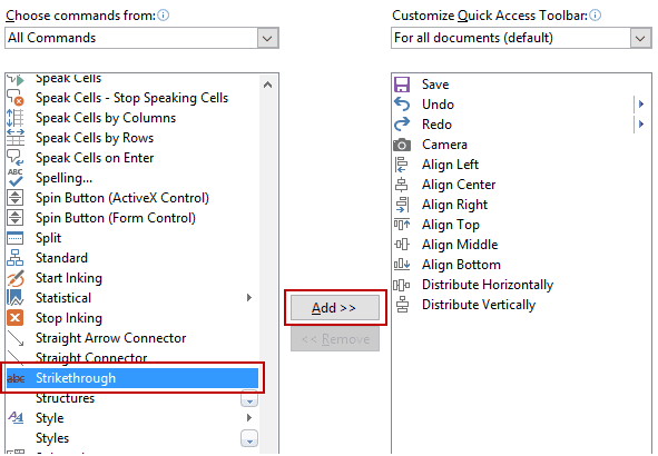 591×410 strikethrough excel cell keyboard shortcut examples from trumpexcel.com
  474×276 strikethrough excel goskills from www.goskills.com
 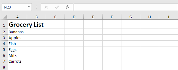 604×238 strikethrough excel easy shortcut from www.excel-easy.com
  356×301 strikethrough excel examples strikethrough from www.educba.com