Best Excel Formula For Checking Duplicate Entries
Finding Duplicate Entries in Excel: A Comprehensive Guide
Excel’s vast capabilities extend far beyond simple data entry. One of its most valuable applications is identifying and managing duplicate entries within your spreadsheets. Whether you’re working with customer lists, inventory records, or any other dataset, duplicates can skew your results and lead to inaccurate insights. This guide explores several powerful Excel formulas and techniques for effectively detecting and handling duplicates, specifically within datasets containing a large number of rows (e.g., 1000+).
Understanding the Importance of Duplicate Removal
Before diving into the formulas, let’s understand why eliminating duplicates is crucial:
- Data Accuracy: Duplicates distort calculations like averages, sums, and counts, leading to flawed reports and analyses.
- Data Integrity: Maintaining data integrity ensures consistency and reliability, essential for making informed decisions.
- Storage Efficiency: Removing duplicates reduces file size and optimizes storage space.
- Improved Efficiency: Working with clean data streamlines processes and reduces the risk of errors.
- Better Reporting: Accurate reports based on de-duplicated data provide a clearer and more representative view of your information.
The COUNTIF Function: Your Go-To Solution
The `COUNTIF` function is the workhorse for duplicate detection in Excel. It counts the number of cells within a range that meet a given criterion. In our case, the criterion will be whether a value appears more than once in the column.
Basic COUNTIF Usage
Let’s assume your data is in column A, starting from cell A2 (A1 often holds the header). Here’s the formula:
=COUNTIF($A$2:$A$1000,A2)
Explanation:
COUNTIF(range, criteria): This is the basic syntax of the function.$A$2:$A$1000: This is the range where you want to search for duplicates. The dollar signs ($) are crucial. They create an absolute reference, meaning the range will not change when you copy the formula down. This ensures you’re always comparing against the entire dataset. Adjust ‘1000’ to match the actual last row of your data.A2: This is the criteria – the value you’re looking for within the range. It’s a relative reference. When you copy the formula down, A2 will change to A3, A4, and so on, comparing each cell’s value against the entire range.
How it Works: The formula in cell B2 (next to A2) counts how many times the value in A2 appears within the range A2:A1000. Copy this formula down to cell B1000. If the value in column B is greater than 1, it indicates that the corresponding value in column A is a duplicate.
Interpreting the Results
After applying the `COUNTIF` formula, you’ll have a column indicating the frequency of each value. You can then use this information to:
- Filter: Filter the column with the `COUNTIF` results to show only values greater than 1. This will display all the duplicate entries.
- Conditional Formatting: Use conditional formatting to highlight the duplicate entries directly in column A. Select column A, go to “Conditional Formatting” -> “Highlight Cells Rules” -> “Duplicate Values”.
- Create a New Column for Flagging: Create a new column (e.g., column C) with a formula to explicitly flag duplicates:
=IF(COUNTIF($A$2:$A$1000,A2)>1, "Duplicate", ""). This will display “Duplicate” in column C for all duplicate entries.
Beyond Basic COUNTIF: Handling Complex Scenarios
The basic `COUNTIF` works well for single-column duplicates. However, you might need to identify duplicates based on multiple columns (e.g., first name, last name, and email address). Here’s how to handle such situations:
Concatenation: Combining Multiple Columns
One approach is to concatenate the values from multiple columns into a single column and then use `COUNTIF` on the concatenated column.
Example: Let’s say you want to identify duplicates based on columns A (First Name), B (Last Name), and C (Email). In column D, enter the following formula (starting from D2):
=A2&B2&C2
This formula combines the values from A2, B2, and C2 into a single string. Copy this formula down to D1000. Now, use the `COUNTIF` function on column D, similar to the previous example:
=COUNTIF($D$2:$D$1000,D2)
Apply this formula to column E (starting from E2) and copy it down. You can now filter or highlight based on the values in column E.
Important Considerations for Concatenation:
- Separators: When concatenating, use separators to avoid false positives. For example, if A2 is “John” and B2 is “Smith”, and A3 is “JohnS” and B3 is “mith”, without a separator, A2&B2 and A3&B3 would both result in “JohnSmith”. Use a separator like this:
=A2&"_"&B2&"_"&C2. A common separator is “_”, “-“, or even a pipe “|”. - Data Type Consistency: Ensure that the data types in the concatenated columns are consistent. For example, if one column contains numbers and another contains text, you might need to format them consistently before concatenation using the `TEXT` function.
Using the `COUNTIFS` Function: Multiple Criteria with Precision
For a more elegant and direct approach to handling multiple criteria, use the `COUNTIFS` function. `COUNTIFS` allows you to specify multiple ranges and criteria, checking if all conditions are met simultaneously.
Example: Using the same First Name (A), Last Name (B), and Email (C) example, the formula in column D (starting from D2) would be:
=COUNTIFS($A$2:$A$1000,A2,$B$2:$B$1000,B2,$C$2:$C$1000,C2)
Explanation:
COUNTIFS(criteria_range1, criteria1, [criteria_range2, criteria2], ...): This is the syntax of the function.$A$2:$A$1000,A2: Counts how many times the value in A2 appears in the range A2:A1000.$B$2:$B$1000,B2: Counts how many times the value in B2 appears in the range B2:B1000.$C$2:$C$1000,C2: Counts how many times the value in C2 appears in the range C2:C1000.
The `COUNTIFS` function returns the number of rows where all three conditions are met – essentially, the number of rows that have the same first name, last name, and email address. If the result is greater than 1, it’s a duplicate.
Advantages of `COUNTIFS`:
- Clarity: The formula is more readable and easier to understand compared to concatenation.
- Efficiency: It’s generally more efficient than concatenating large datasets.
- Directness: It directly addresses the problem of identifying duplicates based on multiple criteria without requiring an intermediate step.
Removing Duplicates: Excel’s Built-in Tool
While formulas are excellent for identifying duplicates, Excel provides a built-in tool for removing them directly. This tool is located under the “Data” tab -> “Remove Duplicates.”
How to Use the “Remove Duplicates” Tool:
- Select the range of cells containing the data you want to de-duplicate. Make sure to include headers if your data has them.
- Go to the “Data” tab and click “Remove Duplicates.”
- A dialog box will appear, listing the columns in your selected range. Check the columns you want to use for duplicate identification. If you want to remove duplicates based on all columns, leave all boxes checked.
- Click “OK.”
Excel will remove the duplicate rows and display a message indicating how many duplicates were removed and how many unique values remain.
Important Considerations for Using “Remove Duplicates”:
- Permanent Changes: Removing duplicates is a permanent action. It’s advisable to create a backup copy of your data before using this tool.
- First Occurrence Preserved: The “Remove Duplicates” tool keeps the first occurrence of each unique row and removes subsequent duplicates. If you need to preserve a specific occurrence based on other criteria (e.g., the most recent entry), you might need to sort your data first.
- Hidden Rows/Columns: The tool operates on visible rows and columns. Make sure any relevant rows or columns are unhidden before running the tool.
Choosing the Right Approach
The best method for identifying and removing duplicates depends on your specific needs and the complexity of your data:
- Simple Single-Column Duplicates: The basic `COUNTIF` formula is sufficient.
- Multi-Column Duplicates: `COUNTIFS` is generally the preferred method due to its clarity and efficiency. Concatenation is an alternative but requires careful consideration of separators and data types.
- Direct Removal of Duplicates: The “Remove Duplicates” tool is ideal for quickly eliminating duplicates after they have been identified. However, always back up your data first.
- Dynamic Duplicate Detection: If your data is constantly updated, formulas (especially using conditional formatting) provide a dynamic way to track duplicates as they are added.
Conclusion
Excel offers a range of powerful tools and formulas for effectively detecting and handling duplicate entries. By understanding the `COUNTIF` and `COUNTIFS` functions, as well as the “Remove Duplicates” tool, you can ensure the accuracy, integrity, and efficiency of your data, leading to better insights and more informed decision-making. Remember to choose the approach that best suits your specific requirements and always back up your data before making any permanent changes.
 700×400 excel formula highlight duplicate values exceljet from exceljet.net
  394×319 prevent duplicate entries excel step step tutorial from www.excel-easy.com
  397×472 find duplicate entries microsoft excel from www.groovypost.com
 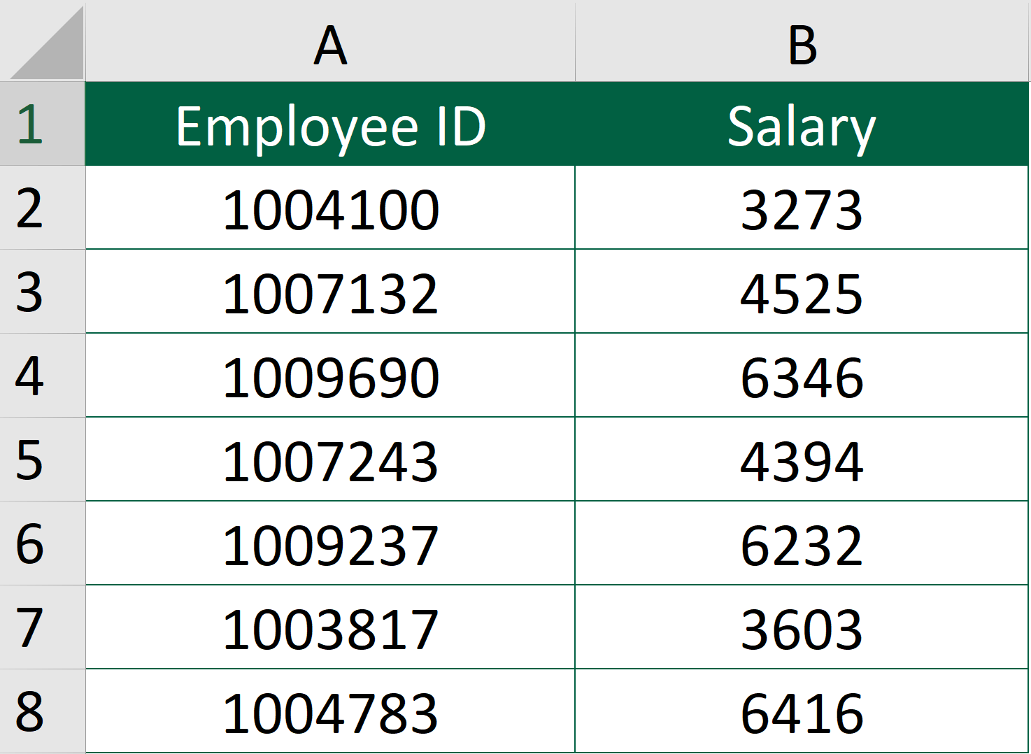 1474×1078 prevent duplicate entries excel dollar excel from dollarexcel.com
 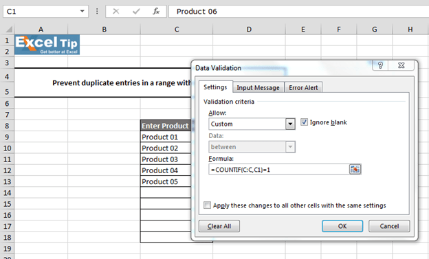 624×377 prevent duplicate entries range excel data validation from www.exceltip.com
  741×480 checking duplicates excel column ngdeveloper from ngdeveloper.com
  650×645 remove duplicate rows excel from www.howtogeek.com
  904×634 onlineoffline earn money easy skills duplicates from oemwes.blogspot.com
  1024×428 find duplicate values excel find search duplicate from yodalearning.com