How To Use Data Tables For What-if Analysis In Excel
“`html
Unleashing “What-If” Power with Data Tables in Excel
Excel’s Data Tables are a powerful, yet often overlooked, feature for performing “what-if” analysis. They allow you to explore how changes in one or two input variables impact one or more formulas in your spreadsheet. This is incredibly useful for financial modeling, sensitivity analysis, and general decision-making. Instead of manually changing inputs and recording the resulting outputs, Data Tables automate this process, presenting a clear overview of different scenarios.
Understanding Data Tables: The Fundamentals
At its core, a Data Table is a range of cells that automatically recalculates formulas based on different input values you specify. Excel offers two types of Data Tables:
- One-Variable Data Table: Examines the effect of changing a single input variable on one or more formulas. This is ideal for understanding the impact of, say, different interest rates on a loan payment or varying sales volumes on profit.
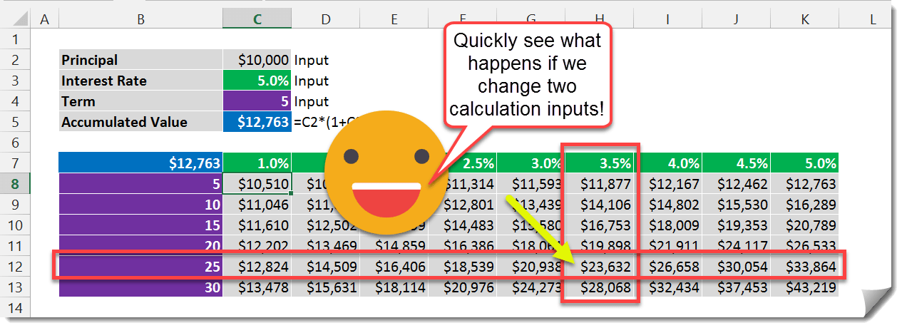
- Two-Variable Data Table: Explores the impact of changing two input variables simultaneously on a single formula. This is useful for analyzing how both price and cost of goods sold affect profit margins or how interest rate and loan term affect monthly payments.
Before diving into the “how-to,” let’s clarify some key terms:
- Input Cell: The cell that the Data Table uses as the input. This is the cell whose value is changing in each scenario. It needs to be referenced by the formula(s) you are analyzing.
- Formula Cell(s): The cell(s) containing the formula(s) that you want to evaluate. The Data Table will calculate the results of these formulas for each input value.
- Table Range: The entire range of cells that comprise the Data Table, including the input values, the formula cell references, and the calculated results.
Creating a One-Variable Data Table: A Practical Example
Let’s illustrate with an example. Imagine you’re analyzing the monthly payment on a loan based on different interest rates. Assume you have the following:
- Loan Amount (B1): $100,000
- Loan Term in Years (B2): 30
- Interest Rate (B3): 5% (This is our input cell, which will change)
- Monthly Payment (B4):
=PMT(B3/12, B2*12, B1)(This is our formula cell)
Here’s how to create a one-variable Data Table to see the impact of interest rates from 4% to 6% in increments of 0.25%:
- Set up the Input Values: In a column (e.g., column D), enter the different interest rates you want to test. Start at D6, and enter 4%, 4.25%, 4.5%, 4.75%, 5%, 5.25%, 5.5%, 5.75%, and 6%. Remember to format these cells as percentages.
- Reference the Formula: In the cell above and to the right of your first interest rate (cell E5), enter a formula that references the cell containing the formula you want to calculate. In our case, enter
=B4. This tells the Data Table which result to display. This cell (E5) will display the initial monthly payment based on the interest rate in B3 (5%). - Select the Table Range: Select the entire range that includes your input values and the formula reference (D5:E14 in our example).
- Open the Data Table Dialog: Go to the “Data” tab on the ribbon, click on “What-If Analysis,” and then select “Data Table…”
- Specify the Input Cell: In the Data Table dialog box, you’ll see fields for “Row input cell” and “Column input cell.” Since our interest rates are arranged in a column, we’ll use the “Column input cell” field. Click in the “Column input cell” field and then click on cell B3 (the cell containing our original interest rate).
- Click OK: Excel will automatically populate the Data Table with the monthly payments calculated for each interest rate.
Now, column E (from E6:E14) will display the monthly payment for each corresponding interest rate in column D (from D6:D14). You can easily see how sensitive the monthly payment is to changes in the interest rate.
Working with Multiple Formulas in a One-Variable Data Table
The real power comes when you analyze multiple formulas with the same input. Let’s extend our loan example. Suppose you also want to calculate the total amount paid over the loan term.
- Total Amount Paid (B5):
=B4 * B2 * 12(Monthly Payment * Loan Term in Years * 12)
To add this to our existing Data Table:
- Add the Formula Reference: In the cell next to your existing formula reference (F5), enter a formula that references the Total Amount Paid cell:
=B5. - Expand the Table Range: Select the entire range that now includes your input values and both formula references (D5:F14).
- Open the Data Table Dialog: Go to the “Data” tab on the ribbon, click on “What-If Analysis,” and then select “Data Table…” (The column input cell B3 should already be populated.)
- Click OK: Excel will update the Data Table.
Now, column E will still display the monthly payments, and column F will display the total amount paid for each corresponding interest rate. This allows you to quickly compare the impact on both key outputs.
Creating a Two-Variable Data Table: Exploring Two Inputs
Let’s say you want to analyze the monthly payment based on varying both the interest rate and the loan term. We’ll use the same setup as before but now vary the loan term in years as well.
- Loan Amount (B1): $100,000
- Loan Term in Years (B2): 30 (One of our input cells)
- Interest Rate (B3): 5% (The other input cell)
- Monthly Payment (B4):
=PMT(B3/12, B2*12, B1)(Our formula cell)
Here’s how to create a two-variable Data Table:
- Set up the Row and Column Inputs: In the first column (e.g., column D), enter the different interest rates you want to test, as before (D7:D15: 4% to 6% in 0.25% increments). In the first row (e.g., row 6), enter the different loan terms in years you want to test (E6:I6: 10, 15, 20, 25, 30).
- Reference the Formula: In the cell at the intersection of the row and column inputs (cell D6), enter a formula that references the cell containing the formula you want to calculate. In our case, enter
=B4. - Select the Table Range: Select the entire range that includes your input values and the formula reference (D6:I15).
- Open the Data Table Dialog: Go to the “Data” tab on the ribbon, click on “What-If Analysis,” and then select “Data Table…”
- Specify the Input Cells: In the Data Table dialog box, click in the “Row input cell” field and then click on cell B2 (the cell containing our original loan term). Click in the “Column input cell” field and then click on cell B3 (the cell containing our original interest rate).
- Click OK: Excel will automatically populate the Data Table with the monthly payments calculated for each combination of interest rate and loan term.
Now, you have a table where each cell shows the monthly payment for a specific combination of interest rate (column) and loan term (row). This gives you a comprehensive view of how both variables affect the outcome.
Important Considerations and Tips
- Formula References are Crucial: Data Tables work by referencing cells containing formulas. Make sure your formulas are correctly set up before creating the Data Table.
- Data Tables are Not Dynamic: While Data Tables automatically recalculate when the source data changes (e.g., the loan amount), they are not dynamically linked to the input values themselves. If you change the input values in the table (e.g., change an interest rate from 4% to 4.1%), the formulas won’t automatically recalculate based on that *change* to the table’s input, you’d have to change the actual input cell and let the table recompute all values.
- Performance: Data Tables can slow down large spreadsheets, especially two-variable tables. Consider turning off automatic calculation (Formulas tab > Calculation Options > Manual) while working on other parts of your spreadsheet and then recalculating the table when needed (press F9).
- Formatting: Format the Data Table cells appropriately to display the results clearly (e.g., currency format for monetary values, percentage format for interest rates).
- Error Handling: If you encounter errors in your Data Table, double-check your formulas and input cell references. A common mistake is referencing the wrong input cell or having an error in the original formula.
- Beyond Loan Calculations: Data Tables are applicable to a wide range of scenarios beyond loan calculations, including budgeting, sales forecasting, investment analysis, and project management. Think of any situation where you want to see how changing one or two key inputs affects one or more outcomes.
Conclusion
Data Tables are a valuable tool in Excel for performing “what-if” analysis, enabling you to explore different scenarios and make informed decisions. By understanding the fundamentals of one-variable and two-variable Data Tables, you can leverage this feature to gain deeper insights from your data and improve your analytical capabilities.
 1265×460 data tables analysis excel from www.howtoexcel.org
 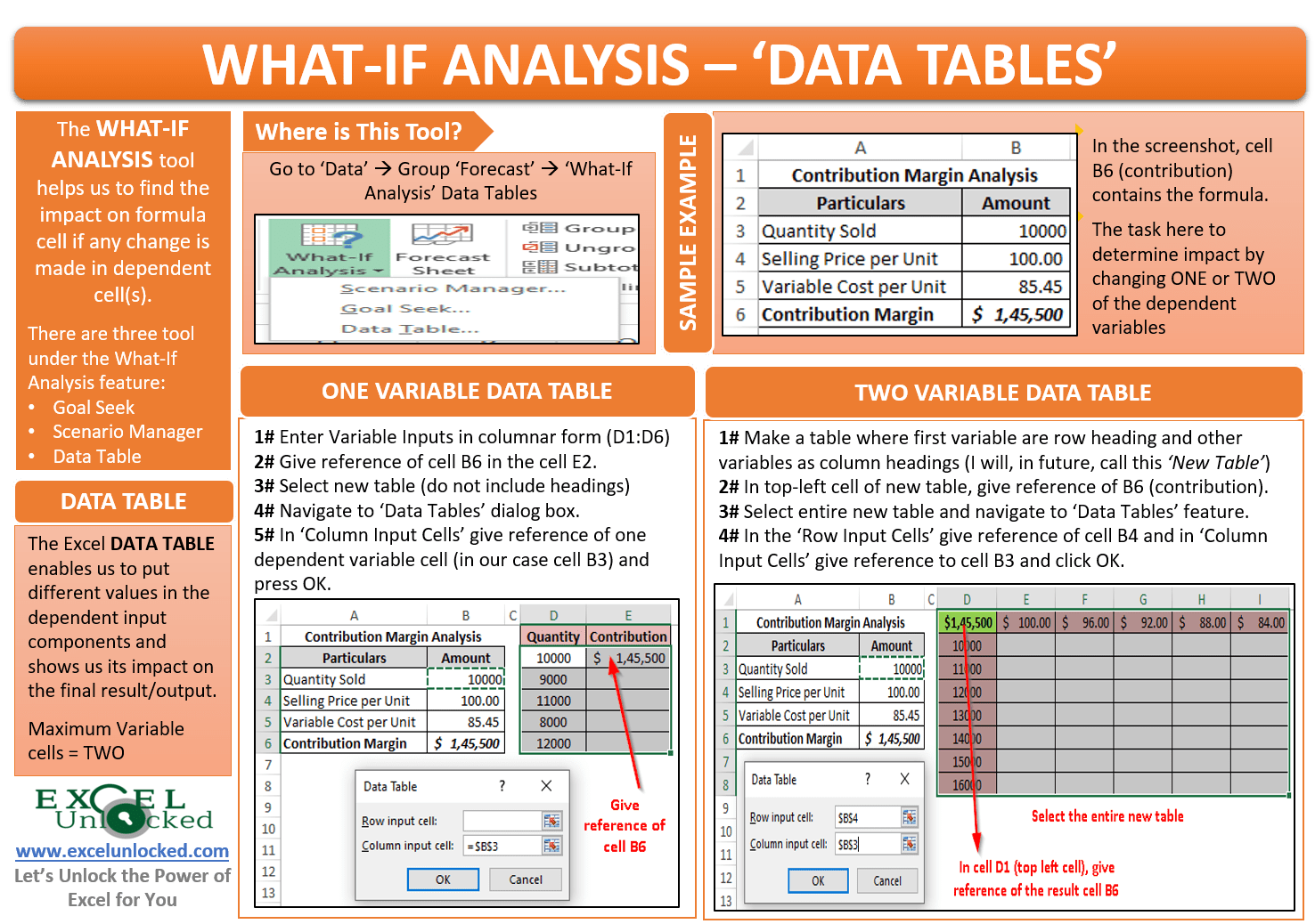 1476×1038 analysis data table excel excel unlocked from excelunlocked.com
  3481×1614 data table analysis excel excel maverick from excelmaverick.com
  800×451 analysis data tables excel chris menard training from chrismenardtraining.com