How To Do ABC Analysis In Excel For Inventory
ABC analysis is a method of categorizing inventory items based on their value and importance. It’s based on the Pareto principle (also known as the 80/20 rule), which suggests that roughly 80% of effects come from 20% of the causes. In inventory management, this translates to a small percentage of items often representing a large portion of the total inventory value. By using ABC analysis in Excel, you can prioritize your inventory management efforts, focusing on the most critical items for better control and optimization. Here’s a detailed guide on how to perform ABC analysis in Excel:
Step 1: Data Preparation
First, you need to gather and organize your inventory data in Excel. The essential data points are:
* **Item Code/SKU:** A unique identifier for each inventory item. * **Annual Demand/Usage:** The number of units of each item used or sold in a year. * **Unit Cost:** The cost of acquiring one unit of each item.
Your data should be organized into columns. For example:
| Item Code | Annual Demand | Unit Cost | |—|—|—| | A100 | 1000 | $10.00 | | B200 | 500 | $5.00 | | C300 | 2000 | $2.00 | | D400 | 100 | $20.00 | | E500 | 3000 | $1.00 | | … | … | … |
Step 2: Calculate Annual Usage Value
The next step is to calculate the annual usage value for each item. This is done by multiplying the annual demand by the unit cost.
- In a new column (e.g., “Annual Usage Value”), enter the formula: `=Annual Demand * Unit Cost`. Replace “Annual Demand” and “Unit Cost” with the actual cell references. For example, if “Annual Demand” is in column B and “Unit Cost” is in column C, and your data starts in row 2, the formula in cell D2 would be `=B2*C2`.
- Drag the formula down to apply it to all items in your inventory list.
Now your table should look like this:
| Item Code | Annual Demand | Unit Cost | Annual Usage Value | |—|—|—|—| | A100 | 1000 | $10.00 | $10,000.00 | | B200 | 500 | $5.00 | $2,500.00 | | C300 | 2000 | $2.00 | $4,000.00 | | D400 | 100 | $20.00 | $2,000.00 | | E500 | 3000 | $1.00 | $3,000.00 | | … | … | … | … |
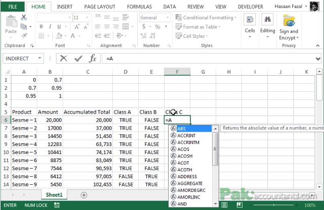
Step 3: Sort by Annual Usage Value
To perform the ABC analysis, you need to sort your data in descending order based on the “Annual Usage Value.”
- Select all the data in your table.
- Go to the “Data” tab in the Excel ribbon.
- Click on “Sort.”
- In the “Sort” dialog box:
- In the “Sort by” dropdown, select “Annual Usage Value.”
- In the “Order” dropdown, select “Largest to Smallest.”
- Ensure “My data has headers” is checked if your data includes a header row.
- Click “OK.”
Your table is now sorted, with the highest-value items at the top.
Step 4: Calculate Cumulative Usage Value and Percentage
Now, calculate the cumulative usage value and the cumulative percentage of the total usage value.
- **Cumulative Usage Value:** In a new column (e.g., “Cumulative Usage Value”), calculate the running total of the “Annual Usage Value.”
- In the first row (e.g., E2), enter the same value as the first “Annual Usage Value” (e.g., `=D2`).
- In the second row (e.g., E3), enter the formula to add the current “Annual Usage Value” to the previous “Cumulative Usage Value” (e.g., `=E2+D3`).
- Drag the formula down to apply it to all remaining items.
- **Cumulative Percentage:** In another new column (e.g., “Cumulative Percentage”), calculate the percentage of the total usage value represented by the cumulative usage value.
- First, calculate the total usage value for all items. You can use the `SUM` function at the bottom of the “Annual Usage Value” column (e.g., `=SUM(D2:D100)` if you have 100 items). Let’s call this cell `D101` for example.
- In the first row of the “Cumulative Percentage” column (e.g., F2), enter the formula: `=(Cumulative Usage Value / Total Usage Value)*100`. Replace “Cumulative Usage Value” and “Total Usage Value” with the appropriate cell references. For instance, `= (E2/$D$101)*100`. The `$` signs are important to make the cell reference for `Total Usage Value` absolute, so it doesn’t change when you drag the formula down.
- Drag the formula down to apply it to all items.
Your table now looks like this (with calculated columns):
| Item Code | Annual Demand | Unit Cost | Annual Usage Value | Cumulative Usage Value | Cumulative Percentage | |—|—|—|—|—|—| | [Highest Value Item] | … | … | … | … | … | | … | … | … | … | … | … | | [Lowest Value Item] | … | … | … | … | … |
Step 5: Assign ABC Categories
Based on the cumulative percentage, assign each item to one of the ABC categories. The typical ranges are:
* **A Items:** Top 70-80% of total annual usage value (approximately 10-20% of items). These are the most critical items. * **B Items:** Next 15-20% of total annual usage value (approximately 30% of items). These items are moderately important. * **C Items:** Remaining 5-10% of total annual usage value (approximately 50-60% of items). These are the least important items.
You can use an `IF` formula in Excel to automatically assign the categories. In a new column (e.g., “ABC Category”), enter the following formula in the first row (e.g., G2), adjusting the percentages as needed:
“`excel =IF(F2<=70,"A",IF(F2<=90,"B","C")) ```
This formula checks the “Cumulative Percentage” (e.g., F2). If it’s less than or equal to 70%, the item is assigned to category “A.” If it’s greater than 70% but less than or equal to 90%, the item is assigned to category “B.” Otherwise, it’s assigned to category “C.” Adjust the 70 and 90 based on your desired thresholds. Drag the formula down to apply it to all items.
Your final table should look like this (with all calculated columns including the ABC Category):
| Item Code | Annual Demand | Unit Cost | Annual Usage Value | Cumulative Usage Value | Cumulative Percentage | ABC Category | |—|—|—|—|—|—|—| | [Highest Value Item] | … | … | … | … | … | A | | … | … | … | … | … | … | A/B/C | | [Lowest Value Item] | … | … | … | … | … | C |
Step 6: Analyze and Interpret Results
Now that you’ve categorized your inventory, you can analyze the results and use them to make informed decisions about inventory management.
* **Count Items in Each Category:** Use the `COUNTIF` function to determine the number of items in each category. For example, to count the number of “A” items, use the formula: `=COUNTIF(G2:G100,”A”)`. Do the same for “B” and “C” items. * **Calculate Percentage of Items in Each Category:** Divide the number of items in each category by the total number of items and multiply by 100 to get the percentage.
Based on the analysis, you can implement the following strategies:
* **A Items:** * Tight inventory control: Frequent monitoring, accurate forecasting, and secure storage. * Negotiate favorable pricing with suppliers. * Consider just-in-time (JIT) inventory management. * **B Items:** * Moderate inventory control: Regular monitoring and periodic reviews. * Maintain adequate safety stock levels. * **C Items:** * Looser inventory control: Simpler reordering processes and larger safety stock levels. * Consider bulk purchasing to reduce ordering costs.
Key Considerations and Refinements
* **Adjust Percentage Thresholds:** The 70/90 thresholds for ABC categories are just guidelines. You may need to adjust them based on your specific business needs and industry. * **Dynamic Analysis:** Set up your Excel spreadsheet to be dynamic. Use formulas and named ranges so that when you update your inventory data (annual demand, unit cost), the ABC analysis automatically recalculates. * **Multiple Criteria:** You can combine ABC analysis with other criteria, such as lead time or supplier reliability, for a more comprehensive inventory management approach. * **Regular Review:** Inventory needs and market conditions change. Perform ABC analysis periodically (e.g., quarterly or annually) to ensure your inventory management strategies remain effective. * **Visualization:** Create charts and graphs (e.g., pie charts or bar charts) to visually represent the distribution of items across the ABC categories and their contribution to the total inventory value. This makes it easier to communicate the results of your analysis to stakeholders.
By following these steps, you can effectively use Excel to perform ABC analysis and optimize your inventory management, leading to reduced costs, improved service levels, and better overall business performance.
 640×416 abc inventory analysis excel charts pakaccountantscom from pakaccountants.com
 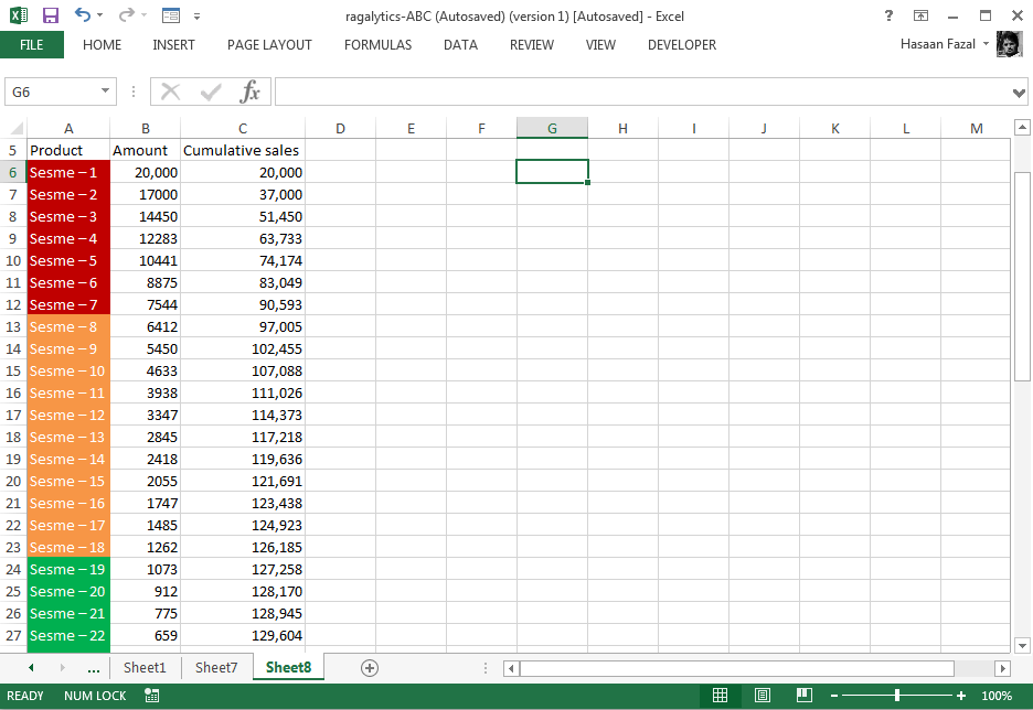 474×326 abc analysis conditional formatting excel pakaccountantscom from pakaccountants.com